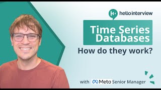

Why Relational DBs Fail for Time Series
46sExplains a common pain point with concrete numbers (50k writes/sec) and promises a solution, hooking engineers.
▶ Play Clip"Delivers a thorough, technical explanation that matches the title, though it could be trimmed slightly."
This video provides an in-depth explanation of how time series databases work, covering the underlying techniques that enable high write throughput, efficient storage, and fast queries. It also discusses when to use a time series database versus a general-purpose database, using a server monitoring example to illustrate the concepts.
Time series databases are specialized for specific write and read patterns. They are not commonly seen in system design interviews due to interviewer unfamiliarity and narrow application.
A fleet of 100,000 servers reporting metrics every 10 seconds results in 50,000 writes per second (best case) and up to 500,000 writes per second (worst case). Relational databases typically cap at around 10,000 writes per second.
Three problems: high write volume, inefficient storage (large timestamps, host names, metric names), and slow queries that require scanning billions of rows.
To achieve high write performance, avoid random seeks. Append-only storage writes sequentially, and LSM trees organize data in memory (memtable) before flushing to disk as segments, with compaction done offline.
Delta encoding stores differences between consecutive values, reducing storage. For timestamps, delta-of-deltas can often be represented with a single bit, as shown in Facebook's Gorilla paper.
Store metadata like time ranges, tags, and min/max values to skip irrelevant files. Bloom filters can efficiently test if a block contains a specific host, reducing space by 10-100x.
Reduce granularity of older data (e.g., minute-level after a week, hour-level after a month) to save storage and speed up queries.
Data is written to a write-ahead log, then organized in memory by series (metric name + tags). On flush, data is compressed and indexed. Queries filter by time and tags, then load and process relevant blocks.
High cardinality (e.g., storing likes per user/post) creates millions of series, breaking the model. Use a general-purpose database like PostgreSQL for such cases.
Time series databases are ideal for telemetry and sensor data with low cardinality. Prometheus, TimescaleDB, and InfluxDB are popular options.
Time series databases are powerful tools for handling high-frequency, low-cardinality data, but they are not a one-size-fits-all solution. Understanding their internal mechanisms helps engineers decide when to use them and when to opt for a general-purpose database.
What are the three main problems with using a relational database for time series data?
High write volume, inefficient storage, and slow queries that require scanning billions of rows.
03:24
What is the typical write throughput limit for relational databases?
Around 10,000 writes per second.
04:20
What is delta encoding?
Storing the difference between consecutive values instead of the raw values, reducing storage size.
16:09
What is the main advantage of using a bloom filter for block-level metadata?
It requires 10 to 100 times less space than a hash set and can quickly determine if a block definitely does not contain a specific host.
23:01
What is downsampling in time series databases?
Reducing the granularity of older data (e.g., minute-level after a week) to save storage and speed up queries.
24:13
What is the 'cardinality' problem in time series databases?
When the number of unique series (metric name + tags) becomes too large (millions or billions), the storage and query model breaks down.
33:29
What is the role of the write-ahead log in a time series database?
It ensures durability by writing data to disk first, so it can be recovered after a crash.
27:18
What is the purpose of the memtable in an LSM tree?
It is an in-memory staging area where data is sorted and organized before being flushed to disk as segments.
12:03
What is the 'Gorilla' paper and what did it demonstrate?
Facebook's Gorilla paper showed that timestamps in time series data can often be compressed to a single bit using delta-of-deltas encoding.
18:48
What are the three popular time series databases mentioned?
Prometheus, TimescaleDB, and InfluxDB.
36:04
Append-Only Storage and LSM Trees
This is the foundational technique that enables high write throughput by avoiding random seeks.
06:52Delta Encoding and Compression
Shows how simple encoding tricks can dramatically reduce storage requirements.
14:59Block-Level Metadata and Bloom Filters
Demonstrates how metadata and probabilistic data structures can speed up queries.
19:34Downsampling
A practical strategy to balance storage and query performance for historical data.
24:13Cardinality Limitations
Highlights the critical constraint that determines when time series databases are appropriate.
33:29[00:02] cover time series databases. Time series databases are super cool and super interesting. In some sense they are hypers specialized for a very specific type of writing and reading patterns that occur not infrequently in
[00:17] production. Now as it relates to system design interviews, you don't often see time series databases for two reasons. One is that interviewers aren't uniformly familiar with time scale or influx DB and secondly that time series
[00:31] databases have a pretty narrow application. There are actually a bunch of places where you might think hey I'll use a time series database but it doesn't actually work for non-intuitive reasons. So in this video we are going
[00:43] to go deep to explain how they work under the covers so that you'll be able to separate those cases that it works and those cases that it doesn't work. The other benefit to us going deep on time series databases is they're
[00:55] comprised of a bunch of relatively simple ideas that when put together make very powerful systems. In the worst case, you're going to get a bunch of interesting tools for your toolbox that might come in handy for some of your
[01:08] lot of ground in this video, but if you prefer in a written format, I will include in the description a link to the article on our website where you can read through some similar content that
[01:21] covers the same ground. Also on hello.com, you can find common problem breakdowns for system design interviews, other technologies, patterns that are going to be relevant, basically everything that you need as a software
[01:34] engineer to help get you ready for your interviews. and also we've had a lot of engineer afterwards. So definitely go start with an example that should be familiar to most engineers. Let's
[01:47] pretend we maintain a fleet of servers and we're a big company like Airbnb or and we're a big company like Airbnb or Meta. So we've got say 100,000 servers and every few seconds we can choose a frequency let's just say 10. Those
[02:01] servers are reporting their CPU utilization, their memory, their disk IO to some central service or database. And we want to store this information so that we can answer questions. This might be the on call engineer asking what's
[02:15] the load on my web servers or it might be someone in finance who's trying to project how many servers we're going to need in the next year. This could also be a higher frequency query pattern where maybe an alerting system is
[02:27] constantly asking, did the load on any of my web servers exceed 80%. And if so, I need to go kick off some alarm. So, we've got this really interesting box you're a brand new engineer, you might be thinking to yourself, I know what
[02:42] I'll do. I'll put a database in here. And so, maybe we can put my SQL into this box. And we're going to need to define some sort of table structure. So maybe we will create a table called metrics. We'll have a column for the
[02:56] timestamp. That might be just a timestamp type column. We'll have the host that's reporting it. This will be the server name. We'll have some sort of metric name. So this might be CPU or memory. And then we'll have the value.
[03:09] This could be a double. This could be a an integer column. Kind of doesn't matter. But this could represent our data. And so the big question is like why does this not work? And this doesn't work for three reasons. The first reason
[03:24] is we've got a lot of write volume that's happening here. So with our that's happening here. So with our 100,000 servers, we are including five metrics. So we've got CPU, memory, input, output, and network. And then
[03:39] we're doing that every 10 seconds. So in this case, we are doing 50,000 writes per second in kind of the the best case. This is assuming these servers are all
[03:51] evenly spreading out their metric reporting. And that's not a very good here. That would be pretty sensible to avoid lining up. But the worst case scenario would be all of those servers report their metrics at the exact same
[04:05] time. And in that case, we have to handle 500,000 writes per second. So this is bad. In general, relational databases usually cap out around 10,000 writes per second. Now, of course, we could shard this. We could have one
[04:20] MySQL instance that was just CPU and one for memory and one for I/IO, but that's kind of impractical. It's pretty expensive already. The next problem that we have is this metrics table isn't very efficient with storage. Basically, this
[04:35] time stamp column is several bytes. The host name is quite large. Maybe it can be a pointer to a string table, so we can save some memory, but by default, most relational databases aren't going to do that. Our metric name similarly
[04:48] needs to be some sort of string. And our value if it's a double is going to be value if it's a double is going to be eight bytes. And so quickly with this 50,000 writes per second, we're going to have 50,000 rows being generated. We are
[05:01] going to start to accumulate billions of records into our database. Now that's not necessarily a problem. Relational databases can store this data. They use diskbased mechanisms, but it's expensive. It is certainly not the most
[05:14] optimal way to store this. And the last problem is somewhat of a deal breaker. When we want to go and query what's the load on my servers, we can write SQL queries. So we could say go select, you know, average of value from metrics
[05:30] know, average of value from metrics where uh metric name is equal to CPU. And that would tell us what's the load on my web servers. But the problem is it would need to go and look at billions of rows in order to answer that question.
[05:45] instead of returning in milliseconds which we would love are taking many minutes. And if we're doing this really frequently we are also wasting CPU and
[05:57] resources that need to be used by this massive number of writes per second. So basically a relational database is not the best solution for this problem and
[06:09] this is the genesis for time series databases. So we really have three problems that we need to tackle. We need to support massive amounts of writes that are happening at high frequency. We need an efficient way to store this data
[06:22] so that way we're not wasting a bunch of space. And then we need a way of storing space. And then we need a way of storing this so that we can answer queries very quickly of the style. Usually filtering by some sort of criteria and then taking
[06:37] an average or getting a full time series over a period. Time series databases are optimal in those cases where we're looking at a one particular or a few time series and trying to make sense of them. So how can we do this? Well,
[06:52] there's a number of tricks that we can employ in order to solve each of these problems. And I want to talk about each of these tricks in isolation before we come back to pull this all together and talk about what the solution is for the
[07:06] majority of time series databases. The first thing that we need to address if we want high write performance is we need to avoid random accesses of memory. Computer architecture is built such that contiguous blocks of memory are the unit
[07:22] contiguous blocks of memory are the unit of currency. If we need to go and grab a random piece of memory from RAM or from disk, things are very slow. Let me talk about how this works on a hard disk really quick so you can understand the
[07:37] physical architecture and then we can talk about how appendon storage prevents us from having to make these random reads and writes. So, a spinning hard disk looks a bit like this. It's a big circle of magnetic platters. They're
[07:51] usually stacked one on top of the other. And then there is an arm here that is And then there is an arm here that is basically reading. It has a read head from this disc. And what happens if I need to grab data from across the disc
[08:05] is this arm actually moves across the platter. So, this allows me to target basically different circles of these spinning platters. The platters are spinning very fast. Most hard discs are somewhere between 10,000 and 15,000 RPM.
[08:21] But moving this arm is not a fast operation. Even though hard discs have been optimized to hell, most hard discs aren't going to be able to do more than aren't going to be able to do more than 100 to 200 different seek operations per
[08:35] second, which is basically when we need to move this arm. And so what you typically see as a result of this and this idea applies to solid state discs as well. Although it's not a physical arm that's moving. It's a consequence of
[08:51] how basically each of the memory modules is laid out. It will always be faster to read contiguous blocks is that you want to avoid these seek operations. So the
[09:03] worst case scenario if we want fast write performance is we have something like this where when we go to write our first item we write it to this location and then when it comes time to write our second item it's actually on a different
[09:18] part of the disk. We need to move the ARM or seek inside of our disc before we can start that write operation. And then for our third item we have to do the same thing. This also applies for the reads for what it's worth. We don't want
[09:33] to have to do that seek on the read side either. Uh what is much faster is instead having all of this memory be contiguous. So my first block that I write, I write to the location at where my head is right now. And then I keep
[09:50] moving that arm across the platter until I get to the second location. And I can start writing uh bites there. and then I keep moving along into the third uh location. I'm basically avoiding all of these seek operations. Now, what does
[10:06] this look like in practice? How do I make sequential writes to disk? Well, the way to do this is to utilize appendon storage. If instead of making edits and updates that might require me to go and move around inside of memory
[10:20] and find that second item and read it and then change it and then write it again. Instead, I'm only going to be just writing, and I'm going to forget about what I wrote before because I'm only going to keep adding to the
[10:34] storage. This allows me to take maximum advantage of the right throughput of my underlying hardware, but it makes it a little bit more complicated. If I do my rights like this in an appendon fashion, how do I organize my data? How can I
[10:50] make sure that I can read it back in an efficient and fast way? Well, that you are probably jumping out of your seat saying LSM trees, LSM trees. And you're totally right. The solution here if we want to maintain some organization
[11:05] of our data is basically to keep a buffer where we can organize small portions of our data or segments of our data before we write it to the disk. So, how does an LSM tree work? Well, typically what happens is when you have
[11:21] an incoming write, the first thing that goes on is we we take that write and we try to flush it to disk in as raw form as possible. We want to make sure that we keep track of that, right? And once we've written it to something like a
[11:35] write ahead log, then we can tell our users, hey, we've received it. We're not going to forget about it. If our system crashes after we've written to the write ahead log, but before we've done some processing, we can always recover and
[11:49] then read from our write ahead log to figure out what did we miss? What was it that we wrote to disk right after we got it, but actually wasn't incorporated into the data structures that actually represent our database. After we've
[12:03] written to the write ahead log, we're going to write to an in-memory structure that is typically referred to as a mem table. And the idea behind a mem table is it's like a staging area for ranks. A
[12:16] mem table gives us the opportunity to do things like sorting and organizing the data. If we want to go and create indexes on individual components, like if we wanted to have an index on the tags that were associated with our data,
[12:31] we'll get back to this in a minute. We can do that before or during the creation of this in-memory data structure. But this is when things are malleable and fluid in our mem table. If we want to reorder things so that way
[12:47] the sorting is maintained or if we wanted to delete things, we can do that wanted to delete things, we can do that in the mem table. But once these items either become big enough or once enough time has passed, we're going to want to
[13:01] persist these or flush them to our disk. So each of those mem tables will be written into segments. And these segments are basically contiguous sequential representations of these mem tables. They basically are the units
[13:18] that we're now working with on disk. The idea behind log structure merge trees is basically we give ourselves some time to organize the data, but we're always writing it in the same appendon fashion, one segment after another. The only
[13:34] exception to this is something that is sometimes called compaction where we might go and look at two segments and say, "Hey, it would actually be beneficial if these two segments were merged together." In that case, an
[13:48] offline process will read segment one. It'll read segment two. It'll write a third segment that is the combination of the first two. And then it will earmark these guys and say, "Hey, they've been deleted." Or we might create some
[14:02] additional entry that tells our system that we should ignore those previous segments. But this compaction doesn't take place on the critical ride path. It takes place in an offline setting where we have more data to work with and we
[14:16] can make sense of whether segments ought to be combined or destroyed or other things that might need to happen. But log structured merge trees give us the best of both worlds. It gives us the appendon sequential write performance
[14:30] that we desire, but it also gives us a chance to organize the data on disk so we're going to read it back. Now I'm handwaving a bit around the middle section here. What's going on in these mem tables? How are we organizing our
[14:44] data before we write it such that it is more optimal for our time series use cases? Let's talk a little bit about what that looks like. One of the most important things that we can be doing in memory for a time series database is
[14:59] finding out some compressed way to represent the information both a to save on storage but b to facilitate fast lookups. Let's talk about the storage
[15:11] for just a second. So when we have time series data, we typically have what are called series. And these are values that are observations taken at specific are observations taken at specific times. And so maybe I have a temperature
[15:26] gauge set up outside my house. And every 10 seconds I pull that temperature gauge and then write it into my database. Now I've got a bunch of timestamps for when I did that and then the value which is the associated temperature. If you look
[15:40] at this naively, how would this data be represented? Well, each of these time stamps would need to be an int. So, four bytes per and then each of these values could be a float or a double, maybe four or eight bytes depending upon the
[15:54] architecture in the system. So, we're using quite a lot of data to store this and the question is well can we do better? And the answer is is yes. One of the simplest approaches that we can do is what's called delta encoding. And the
[16:09] idea behind delta encoding is pretty simple. For a lot of time series data, the values are not going to change dramatically from observation to observation. Maybe I drop that temperature sensor,
[16:23] you know, into a bucket of water just to test its calibration, and I clearly want to know about that when it happens. But for the most part, this isn't going to move a whole lot. So instead of storing the raw values which is kind of the
[16:37] series that I have here, what I can do is store the difference from the previous observation. So my first observation was 56.7. We'll just take an implicit zero as the null observation. So my first delta is
[16:53] null observation. So my first delta is 56.7. From zero, it goes up. My next observation is 58.4. That's a difference of 1.7 from 56.7. So instead, I'm just going to store plus 1.7. If I wanted to know what the value
[17:09] is, I need to go for find the previous value and add 1.7 to it in order to recover. But you'll note that this delta encoded series is substantially smaller. And if you know anything about how computers represent numbers, the smaller
[17:25] the number is, the less bytes that are required for us to store it. So maybe required for us to store it. So maybe instead of taking eight bytes for us to go store a double length value, maybe we are only using two or one bite to store
[17:42] each element of this delta encoded sequence. Now tricks like delta encoding can be applied kind of recursively. One observation here is that timestamps are pretty big. These are integers. They're four bytes long for seconds. And we are
[17:59] typically taking these observations on a really regular cadence. For my my temperature gauge outside, I'm doing this every 10 seconds. So if I went encoding, I would end up with a sequence like this. That would be 10 10 10 10.
[18:17] And using that same logic, we can look at the delta of the deltas that we have. The first delta of deltas is the difference between my null value and my first delta. That's 10. And then every subsequent delta of deltas is just the
[18:33] difference between these two. So this is 0 0. What you see here is a sequence 0 0. What you see here is a sequence that is very easy to compress. Facebook has a famous gorilla paper about a monitoring system that they had built.
[18:48] And what they noticed is that these timestamps could often be represented with as much as or on average a single bit that these zeros are very compressible and substantially more compressible than the 32 bits that I
[19:03] compressible than the 32 bits that I need to store the raw timestamps. So in memory I can take data as long as I have access to previous observations and come up with a substantially more efficient representation of the data before I go
[19:19] and flush it to disk. Now while storing compressed time series data is clearly really important to a time series database, it's not the only trick that we use before we write to disk. Another thing that we can take advantage of is
[19:34] that when we're about to flush to disk, we can store some metadata alongside the batch of data that we're about to write that will help us when it comes time to read. To give you an example of of how this might work, imagine that I'm
[19:49] this might work, imagine that I'm storing server monitoring data. And the use case that frequently comes up for this is I log into Graphfana and I want to look at the last 8 hours of say request volume to figure out whether the
[20:03] web servers are failing because my requests have skyrocketed. It's Black Friday or something else is going on. So when I make that query for the last 8 hours, the worst case scenario would be I have to read all of the data in my
[20:18] database in order to answer it. That's clearly intractable. So timebased partitioning works pretty simply. When we are writing data, we're typically we are writing data, we're typically writing a range of times. Maybe we're
[20:31] writing all of the data for yesterday, which happens to be the 29th on my side. Or maybe we're writing data for today. And when we're writing this data, we can store the interval that is contained. So when I want to go query the last 8 hours
[20:45] when I want to go query the last 8 hours of data and today is the 30th, I know that I only need to query data that was written which contains the last 8 hours. I don't need to read from files that I wrote yesterday because they can't
[21:00] possibly contain data that is relevant for me. That's timebased partitioning in for me. That's timebased partitioning in a nutshell. And this idea extends beyond just time. Imagine that I wanted instead of looking at all requests along across
[21:14] my web servers, I wanted to look at requests that were being received by host one. If I wrote to separate files or separate parts of files, or separate parts of files, hosts one and two versus three and four,
[21:29] then I know that if I want the data for host one, I don't need to read the data from the file that contains host three and four. So the more metadata that I can store that might be relevant for filtering, the more likely I am to have
[21:45] filtering, the more likely I am to have a speed up on the query side when I can ignore data that's not relevant for my query. A final example of this block level metadata would be to store the min and max of a time series. Let's pretend
[21:59] I want to know when errors spike, but errors are generally hovering around errors are generally hovering around zero. If I only look at files where the max is greater than zero, then I can ignore all those files that definitely
[22:13] don't have any errors occurring. So this same idea applies also the values themselves. That's the idea behind block level metadata in query planning. Now when I have this metadata, sometimes it can get big. If I'm recording monitoring
[22:29] for a fleet of a 100,000 hosts, the worst case scenario would be that I have a gigantic list of the hosts that are contained in a specific file. Maybe I have a 100,000 entries. And when I want to decide whether I need to read from
[22:46] that particular file or that particular block, I need to read all of those hosts and then filter down to only the hosts that I care about. Another way for me to store this data is using a bloom filter. A bloom filter is a special data
[23:01] structure which works like a set except a set will tell us whether an item is in the set or out of the set. A bloom filter will tell us the item is definitely not in the set or it might be in the set. It's a probabilistic data
[23:17] structure, but it saves space in that it requires 10 to 100 times less space than the equivalent hash set. And so if we're storing host information in our metadata
[23:31] and we're constantly doing queries that test whether a block contains a given host, it may actually be the case that we should store the hosts as a bloom filter and then we can ask the bloom
[23:45] filter and then we can ask the bloom filter does this file contain the host that I'm looking for and the bloom filter will either say definitely no in which case we can ignore that file file or it'll say maybe it might be here in
[23:59] which case we'll have to read the file in order to find out whether it actually contained it. That would be another optimization we could employ here. The last optimization that we can consider on the right side is downsampling. Often
[24:13] times when we have telemetry data, we're recording it all the time. Maybe I have CPU information that's recorded every 10 seconds, but it's very unlikely that I need to look at the 10second granularity of data 1 year ago. So most time series
[24:31] databases are going to have some sort of downsampling functionality where I can say if the data is older than a week, I only care about a minute grain. And if it's older than a month, maybe I only care about the hour grain. That means
[24:45] I'm storing a lot less data and it also means my queries are going to be tremendously faster because I don't need to pull all the data. It's not as granular. It's not as accurate, but it's going to be more economical and more
[24:59] performant. And the way that this works in most time series databases is we are going to write the granular data to our disk and then periodically we're going to read that data down sample it either randomly or interpolation and then write
[25:15] new data that represents that down sample data and then often times deleting the old data in its place so that way we can only use the new data. All of these approaches are basically going to enable us to have faster reads
[25:31] by taking on some of the work up front as we're writing to disk so that the data is stored in a more optimal fashion that allows us to read more quickly. Now underlying tricks, let's talk about how we can use them to construct a time
[25:47] series database. For a time series database, the data often times looks like this. We've got some sort of metric name and associated tags for a data point. Those tags can really be anything. If this was a server fleet, it
[26:02] might be host names and regions. If these were sensors, we might have a model number and a serial number for the sensor. But these tags are really the ways that we can filter down the data. So choosing the right tags or at
[26:19] least including the right tags is going to be really important if we want to slice and dice our data. For each metric name and associated tags, we're going to have a set of fields. You might think of the fields as a single value, a scalar
[26:34] value. Maybe this is the CPU usage for that server at this particular time. But you wanted that additional data. Maybe we don't only want the aggregate CPU across the server. Maybe we also want to
[26:48] across the server. Maybe we also want to record the per core CPU usage. Maybe and most importantly, we need a timestamp associated with each data point. So the real data will look something like this where we have metric
[27:01] something like this where we have metric names and a set of tags, a value or a field and timestamps that are flooding in often times at millions of entries per second. All of this data is going to stream over to my time series database.
[27:18] happen in my time series database is I'm going to write it to my write ahead log. Basically I'm going to push it to disk. So if my server crash, I can go and retrieve it from that write- ahead log and make sure that I'm actually able to
[27:31] query it later. After I've written to my write- ahead log, then I'm going to start to build my internal in-memory data structures. And one of the most important aspects of that in-memory data structure is organizing all these data
[27:45] structure is organizing all these data points in order by series. So each time I have a data point with a unique metric name and set of tags, I'm going to have a unique series. It's possible for my data to come out of order. Maybe I've
[27:59] got a timestamp from one server that comes in slightly later, but the timestamp is actually earlier than data that I received from another server. So, I want to keep all of these data points sorted in memory keyed by whatever tags
[28:16] and metric name that I have available. That's going to represent my series. On occasion, I'm going to flush that out to disk and that will be configurable by the database. I might do this when the file grows to a gigabyte. I might do
[28:31] this once a day. I can choose when I want to write this out to disk. But when I write to disk, then we're going to go employ some of the compression and encoding that we had talked about earlier. For each series, which is now
[28:44] earlier. For each series, which is now my ordered data points, I'm going to encode them in whatever way is appropriate. So maybe I'll encode my timestamps using delta of deltas. And then I might encode my actual value
[28:58] series using Exor or some sort of delta encoding. And I'm going to write those encoding. And I'm going to write those values into the the file. The file is also going to store some sort of index. And that index is going to tell me which
[29:13] of these series is associated with what tags and metric names. This is basically like a lookup table. So I know where to get the data that's going to be relevant for the queries that I have. Now when it comes to query time, you might have a
[29:29] specialized query language. So like Prometheus has PromQL or we might have an API that can be used but these queries are going to specify filtering criteria and then maybe operations that
[29:43] we perform on the series. So if we get a query like this where we are trying to get the mean CPU usage for servers in US west in prod between two time points the first thing that we're going to do is find out which data files are relevant
[29:59] for those times. So we only need to look at a subset of all the files that we've written to disk. If we're only looking at the time over the last couple days we don't need to pull something from last year. In each of those files, we're
[30:12] immediately going to go to the index and try to figure out which series or blocks are going to be relevant for the query. In this case, since my region is US West and my environment is prod, I can go and look at each of these and try to figure
[30:25] out whether it applies. So the first one does, so I need to include block zero or series 1. The second one does too, so I have to include block one. The the third entry here is in US East, so that doesn't apply. So I don't even need to
[30:39] read this data. And the last block, block three, is my staging environment. So I also don't need to read that data. So my next step is to go look at the blocks that apply. That's block zero and block one. I'm going to go need to load
[30:54] up the timestamps and the values. I'll need to decompress or decode these values because they're stored in a compressed way. I'm going to do that as I read them off. And then I'm going to do any post-processing on that. So if I
[31:09] wanted the mean of the values here, then I'm going to take all of those values, average them, and then return them back to my user. What we've described is the to my user. What we've described is the happy path of a time series database.
[31:24] We're basically exploiting the time series nature of the data, storing the data in contiguous blocks on disk and then including relevant indexes so we can make our queries really fast. All of this sounds really great and you might
[31:39] think well there's a lot of ways that I can represent my data as a time series. As one example let's pretend that we wanted to store likes data in this way. When a user likes a post, maybe I will set the value equals one for the like
[31:56] that happened at that moment by that user and that post ID. Can I use a time series database now to answer questions like can I look at likes over time for a specific post? And this comes back to the cardality assumptions of the tags
[32:15] that we have for a given data point. How does this start to break in our time series database? Well, when we receive the right and write it to the write ahead log, we don't have any problems because we've stored the data as simple
[32:28] as possible. But when we start to go to our mem table, here's where we start to see the cracks because remember, we're storing data in our mem table according to each of the series. And a series is a unique metric name and set of tags
[32:43] associated. So we're now going to have one series for every user post combination. We are going to have trillions of series. Maybe those don't
[32:56] all happen all at once. Um maybe over a few seconds in our me table, we'll only see millions, but we're already straining the the model. when we go to flush to disk now we have to write millions of series and we have millions
[33:12] of entries in our index which is going to be terrible. And then finally when we go to actually do our query we have deep looks into very large indexes and we need to accumulate across billions of series in order to materialize our final
[33:29] time series. So the problem with time series databases often deals with the series databases often deals with the cardality or the number of unique values for the series that we're recording. It's really important that we include in
[33:43] our tags and in our data anything that we might want to filter by. But there are some fundamental limitations to all that we can include. If we include identifiers that have a lot of unique values, that means we're going to have a
[33:58] lot of series and that's going to break our execution and storage model. So, time series databases work really well when we want to pull data from one or a
[34:11] small number of series and do some operations and querying against it. It doesn't really work when the number of series grows into the millions or billions. At that point, you're going to want to use a more general purpose
[34:26] want to use a more general purpose solution like Postgress, Reddus, etc. here, so I wanted to quickly summarize before we wrap things up. We first covered a bunch of tricks that are necessary to make time series databases
[34:39] effective. First of all, we covered appendon storage and LSM trees which write throughput that's required for these systems. Secondly, we covered delta encoding and compression which basically allows us to optimize the disk
[34:53] storage that's required. And finally, we used a bunch of techniques to make the queries faster from timebased partitioning and bloom filters that basically allow us to choose which parts of which files so that we minimize the
[35:06] amount of aggregate reading we need to do in order to answer our users queries. this is implemented under the covers from receiving data and writing it to individual files all the way through to the queries that come in and how we read
[35:21] indexes and load up series so that we can answer those users queries. And along the way we discovered a few things. First of all, when we should avoid time series databases like when our input has really high cardality or
[35:35] when we don't have an implicit timebased filter or dimension which means that time series databases end up being applicable for those cases where we have a small number of series queries involving a time dimension and then
[35:49] often aggregating or doing some processing across time. These are frequently places where we've got measurements that are coming in from external sensors or we're doing telemetry. Those are both great cases
[36:04] where you would use a time series database. In terms of practical series databases that are out there. Prometheus is a very popular observability backend and it has an internal time series database that
[36:19] allows you to aggregate metrics across a fleet of servers. We'll probably talk about it in a future deep dive. Time scale is a Postgress extension which allows Postgress to store time series data in a more optimal format. I would
[36:33] highly recommend it given how often we are recommending Postgress in various solutions. It's kind of a bolt-on solution that allows you to extend Postgress to the time series domain and influx DB often times gets brought up as
[36:47] another alternative if you have a time series use case that's not metrics and monitoring and then can't be solved with a Postgress extension. That would be one that you might look at. If you've got any questions, feel free to visit the
[37:00] be a little bit easier for you to understand what's going on. Happy to answer questions in the comments and you for spending time with me today and
[37:12] you for spending time with me today and looking forward to the next video.



⚡ Saved you 0h 37m reading this? Transcribe any YouTube video for free — no signup needed.