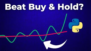

The Dirty Secret of Buy & Hold Investing
44sChallenges a common investing belief with a shocking claim about hidden risk, instantly grabbing attention.
▶ Play Clip"Delivers exactly what the title promises—a clear, code-driven proof of volatility targeting. No fluff, just substance."
This video explains volatility targeting, a risk-based sizing strategy used by hedge funds, and demonstrates how to implement it in Python. The core idea is to scale exposure down in volatile markets and up in calm ones, aiming to keep risk constant. The presenter shows that this simple tweak can improve Sharpe ratios and reduce drawdowns compared to buy-and-hold.
Buy-and-hold risk varies: low in calm years like 2017, high in crises like 2008 or March 2020.
Volatility targeting scales exposure down in chaos and up in calm, often improving Sharpe ratio and reducing drawdowns without forecasting.
Realized volatility is estimated with a 20-day rolling standard deviation, annualized by square root of 252.
Position = target vol / realized vol. Example: 15% target / 30% realized = 50% exposure.
Leverage cap (1.5x) prevents unrealistic 3x-4x positions in ultra-calm markets.
Shift 1 avoids look-ahead bias; fillna(0) holds cash before enough data is available.
Scaling up in calm markets is essential; capping at 1x leaves you under-invested where risk-adjusted returns are best.
Trading costs are modeled at 5 basis points per rebalance, as a proxy for spreads and commissions.
Two return streams are built: buy-and-hold (SPY daily returns) and vol-target (position-scaled returns minus costs).
CAGR uses 365 days (calendar years), not 252, because growth is per actual year.
Volatility is annualized by square root of 252; Sharpe is average daily return divided by daily volatility.
Max drawdown tracks the worst peak-to-trough loss on the cumulative return curve.
Results: slightly higher CAGR, better Sharpe, lower max drawdown than buy-and-hold.
Raising target vol to 25% increases CAGR and Sharpe, with a smaller difference vs buy-and-hold.
Volatility targeting is a simple, robust way to keep risk constant and improve risk-adjusted returns, often beating buy-and-hold with just a few lines of Python.
Risk isn't constant
Challenges the common assumption that buy-and-hold means steady risk, setting up the need for risk-based sizing.
Realized volatility calculation
Shows a concrete, code-level method to estimate market risk using a 20-day rolling standard deviation.
01:36Leverage for risk normalization
Explains why scaling up in calm markets is essential, not reckless, for keeping risk constant.
03:47Strategy outperforms buy-and-hold
Provides empirical evidence that volatility targeting improves Sharpe ratio and reduces drawdowns.
08:32[00:00] Hello and welcome. Here is a dirty little secret about the stock market. If you just buy and hold the S&P 500, your risk isn't constant. Sometimes you are barely taking any risk at all, like in 2017 when markets were dead corn.
[00:19] And sometimes you are taking way too much risk, like in 2008 or March 2020 when volatility spiked and your portfolio blew up.
[00:31] That's why hedge funds almost never just buy and hold. They use risk-based sizing. One of the simplest and most powerful is called volatility targeting.
[00:45] The idea is almost stupidly simple. scale your exposure down in chaotic times and scale it up when the market is quiet. And here's the crazy part.
[00:58] Just doing this one tweak with no forecasting, no machine learning, nothing fancy often gives you higher sharp ratios, smaller drawdowns and sometimes even better returns.
[01:12] Let me prove it to you in Python in about 20 lines of code. After importing a couple of necessary libraries, I am setting some parameters here, which I
[01:24] will get to in a couple of seconds. This is just downloading SPY data starting in 2015 and this is calculating daily returns.
[01:36] This is nothing new until now. This is the important part. Starting with this one here, realized. I estimate realized volatility with a 20 day rolling standard deviation and annualize that
[01:55] by the square root of 252. That gives me a daily estimate of how risky the market looked over the last month.
[02:07] And this pause line here is the critical line of code. So let's break that down. vol divided by realized. This is the core idea. If my target vol is 15%, as I defined here,
[02:25] and let's say my realized vol would be 30%, then 15% divided by 30% would be 50%. So I only want half exposure If the realized more is let say 7 percent then 15 percent divided
[02:45] by 7.5 percent would be 200 that means double exposure. Now this replace 0.0 and PNAM avoids
[02:59] dividing by zero during very quiet streaks. And clip 0.0 and leverage cap keeps the position between zero and 1.5x.
[03:14] Without that, in ultra calm markets, the formula might tell me, go 3x or 4x leveraged, which simply isn't realistic.
[03:26] So I'm capping that here at 1.5 leverage. Shift 1 means we always trade to more using today's information so we don't have look ahead bias and 3MA 0 ensures we hold cash before we have enough data to compute volatility.
[03:47] Now you might ask yourself why do I need leverage? What is this about? This is a key point. Volatility targeting is about keeping risk constant, not just cutting exposure when markets
[04:02] are wide. It also means scaling up when risk is very cheap. Let's take two examples. If volatility spikes to 20% and my target is 15%, then 15% divided by 20% is 0.75.
[04:21] So I scale it down to 75% exposure. No leverage needed here. But if volatility collapses to 5%, then 15% divided by 5% is 3.0.
[04:39] So 300%. So to actually run at 15% risk, I need 300% exposure. If I cap myself at 1x, I'm massively under-invested in exactly the calm, stable regime where risk-adjusted
[04:58] returns are best. That's why professional implementations allow some leverage. But always with a cap. In this example, as said, I cap it at 1.5x.
[05:13] It not about being reckless it about keeping risk steady across different environments Next I add trading costs Every change in POS is a rebalance
[05:27] So I compute turnover as the difference of POS and then the absolute and apply a small 5 basis point cost. That's a rough proxy for bidder spreads and commissions.
[05:40] Now, I build two return streams. Buy and holds, that's just the SPY's daily returns, and the VOL target strategy. POS times REB minus the COS.
[05:53] That is the position scaled returns minus COS. So we are comparing two versions of the same underlying asset. One takes whatever risk the market gives you.
[06:05] The other normalizes risk around 15% with a cap at 1.5x. It's just explained.
[06:17] All right, time to actually measure performance. We'll do this in two parts. First, the function to calculate the key metrics, and then some plots to visualize how the strategy behaves compared to buy and hold.
[06:33] Let's start with the steps function. DropNA is just cleaning the return series in case they are missing weightless. And this one is super important. This is the CAGR calculation.
[06:48] Here in this line, yes, I take the total length of the series in calendar years. That's important because CAGR is about how much your money grows per actual year, not per trading day.
[07:01] That's why I divide by 365 something, not 252. Then total and CAGR compounds all the returns together, then annualized it. So CAGR is if you started with $1, what constant growth rate per year would get you to the
[07:21] same final value? Next one is volatility. CRSD is the daily standard deviation of returns. I multiply it then by the square root of 252 to analyze it.
[07:37] Because volatility scales with the square root of time and risk is measured on trading days. And this is simply the Sharpe ratio, that's the average daily return divided by daily
[07:50] volatility annualized tells us how much return we are getting per unit of risk The higher the sharp the more efficient the return And finally a max drawdown
[08:06] I track the cumulative return curve, compare it to the running maximum and take the minimum. That gives the worst peak to through loss the strategy ever saw.
[08:19] Now lets execute this so we see what we actually get in here. And this is actually quite interesting so you see we have the volatility target strategy
[08:32] versus bind holds here so CAGR slightly outperforming the bind holds by a marginal amount here so this doesn't really matter but we got a higher sub ratio as expected than bind holds we got
[08:50] a volatility around the target volatility which totally makes sense we got a lower next drawdown than for the bind hold strategy so this strategy definitely outperforms the bind hold strategy
[09:05] Now what's interesting here is what we just saw but you can of course tweak the parameters here so for instance you could ask yourself what is happening if I scale up the target
[09:20] volatility to 25% then you just execute everything again and then you see the strategy is running even better as expected you're taking more risks here so you're getting a higher CAGR
[09:35] compared to bind hold you are getting a better sharp ratio but this time it is a bit smaller difference between the two then you have a tight volatility again around the past tight
[09:51] volatility and you have a slightly lower maximum drawdown here also an interesting one here I didn't cover that yet. This is the development of your position. So you see you are at 1.5
[10:08] leverage here. Then you go down in leverage. Then you go up again, down, up again. So you see the interesting market faces here, how your strategy or how your positioning is reacting.
[10:21] reacting. Now I hope you found this as interesting as fascinating as insightful as I found this. Let me know your thoughts in the comments below. Play a
[10:34] bit around with that and I thank you very much for watching and looking forward to see you in the upcoming videos. Cheers. Bye. Bye.
⚡ Saved you 0h 10m reading this? Transcribe any YouTube video for free — no signup needed.