Gradient Descent Visualization
52sThe visual analogy of walking downhill to find the minimum makes a complex algorithm intuitive and engaging.
▶ Play ClipThis lecture introduces linear regression, a foundational supervised learning algorithm. It covers the hypothesis representation, the cost function, and two methods for minimizing it: gradient descent (both batch and stochastic) and the normal equation. The lecture also establishes key notation and concepts used throughout the course.
Supervised learning regression problems have a continuous output, unlike classification problems which have discrete outputs.
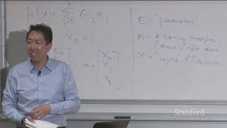
The hypothesis h(x) = theta_0 + theta_1*x_1 + ... + theta_n*x_n, where x_0 = 1 for convenience.
m = number of training examples, n = number of features. x^{(i)} denotes the i-th training example.
J(theta) = 1/2 * sum_{i=1}^{m} (h_theta(x^{(i)}) - y^{(i)})^2. The 1/2 simplifies derivative calculations.
Gradient descent iteratively updates parameters: theta_j := theta_j - alpha * (partial derivative of J w.r.t. theta_j).
Batch gradient descent uses all m examples per update; stochastic gradient descent uses one example per update, making it faster for large datasets.
The normal equation provides a closed-form solution: theta = (X^T X)^{-1} X^T y, where X is the design matrix.
"The title accurately describes the lecture content, which covers linear regression, gradient descent, and the normal equation."
What is a regression problem?
A supervised learning problem where the output variable is a continuous value.
01:22
What is a hypothesis in machine learning?
The function output by a learning algorithm that maps inputs to outputs.
03:28
What does theta represent in linear regression?
The parameters of the learning algorithm.
08:24
What does 'm' represent in the notation used?
The number of training examples.
08:56
What does 'n' represent in the notation used?
The number of features.
11:40
Write the cost function J(theta) for linear regression.
J(theta) = 1/2 * sum_{i=1}^{m} (h_theta(x^{(i)}) - y^{(i)})^2
16:28
What is gradient descent?
An iterative algorithm that minimizes the cost function by taking steps proportional to the negative gradient.
18:04
What does alpha represent in gradient descent?
The learning rate, which controls the step size in gradient descent.
25:01
What is the difference between batch and stochastic gradient descent?
Batch gradient descent uses the entire training set for each update, while stochastic gradient descent uses one example at a time.
41:10
What is the normal equation?
A closed-form solution that directly computes the optimal parameters for linear regression: theta = (X^T X)^{-1} X^T y.
54:42
What is the design matrix X in the normal equation?
The design matrix, where each row is a training example (transposed).
01:08:46
Regression vs. Classification
Clearly distinguishes regression (continuous output) from classification (discrete output), a fundamental concept in supervised learning.
01:22Gradient Descent Intuition
Provides an intuitive, visual explanation of gradient descent as walking downhill, making the algorithm accessible.
18:04Batch vs. Stochastic GD
Explains the practical trade-off between batch and stochastic gradient descent, crucial for handling large datasets.
41:10The Normal Equation
Introduces a closed-form solution for linear regression, highlighting that iterative methods are not always necessary.
54:42Learning Rate Selection
Provides practical advice on choosing the learning rate empirically, a key hyperparameter in many algorithms.
01:18:10[00:03] Morning and welcome back.
[00:06] So what we'll see today in class
[00:10] is the first in-depth discussion of a learning algorithm,
[00:14] linear regression, and in particular,
[00:16] over the next, what,
[00:18] hour and a bit you'll see linear regression,
[00:21] batch and stochastic gradient descent is
[00:24] an algorithm for fitting linear regression models,
[00:26] and then the normal equations, um, uh,
[00:29] as a way of- as a very efficient way to let you fit linear models.
[00:34] Um, and we're going to define notation,
[00:38] and a few concepts today that will lay the foundation
[00:41] for a lot of the work that we'll see the rest of this quarter.
[00:44] Um, so to- to motivate linear regression, it's gonna be, uh,
[00:48] maybe the- maybe the simplest,
[00:50] one of the simplest learning algorithms.
[00:52] Um, you remember the ALVINN video,
[00:55] the autonomous driving video that I had shown in class on Monday,
[00:59] um, for the self-driving car video,
[01:01] that was a supervised learning problem.
[01:04] And the term supervised learning [NOISE] meant
[01:08] that you were given Xs which was a picture of what's in front of the car,
[01:14] and the algorithm [NOISE] had to map that to
[01:16] an output Y which was the steering direction.
[01:19] And that was a regression problem,
[01:22] [NOISE] because the output Y that you want is a continuous value, right?
[01:28] As opposed to a classification problem where Y is the speed.
[01:31] And we'll talk about classification, um,
[01:33] next Monday, but supervised learning regression.
[01:36] So I think the simplest,
[01:38] maybe the simplest possible learning algorithm,
[01:40] a supervised learning regression problem, is linear regression.
[01:44] And to motivate that,
[01:46] rather than using a self-driving car example which is quite complicated,
[01:51] we'll- we'll build up a supervised learning algorithm using a simpler example.
[01:55] Um, so let's say you want to predict or estimate the prices of houses.
[02:01] So [NOISE] the way you build a learning algorithm is
[02:04] start by collecting a data-set of houses, and their prices.
[02:08] Um, so this is a data-set that we collected off Craigslist a little bit back.
[02:12] This is data from Portland, Oregon.
[02:15] [NOISE] But so there's the size of a house in square feet, [NOISE] um,
[02:20] and there's the price of a house in thousands of dollars, [NOISE] right?
[02:25] And so there's a house that is 2,104 square feet whose asking price was $400,000.
[02:32] Um, [NOISE] house with, uh,
[02:34] that size, with that price,
[02:37] [NOISE] and so on.
[02:45] Okay? Um, and maybe more conventionally if you plot this data,
[02:51] there's a size, there's a price.
[02:53] So you have some dataset like that.
[02:56] And what we'll end up doing today is fit a straight line to this data, right?
[03:00] [NOISE] And go through how to do that.
[03:01] So in supervised learning, um,
[03:04] the [NOISE] process of supervised learning is that you have
[03:07] a training set such as the data-set that I drew on the left,
[03:11] and you feed this to a learning algorithm, [NOISE] right?
[03:19] And the job of the learning algorithm is to output a function,
[03:23] uh, to make predictions about housing prices.
[03:26] And by convention, um,
[03:28] I'm gonna call this a function that it outputs a hypothesis, [NOISE] right?
[03:35] And the job of the hypothesis is, [NOISE] you know,
[03:38] it will- it can input the size of a new house,
[03:42] or the size of a different house that you haven't seen yet,
[03:44] [NOISE] and will output the estimated [NOISE] price.
[03:50] Okay? Um, so the job of the learning algorithm is to input a training set,
[03:54] and output a hypothesis.
[03:56] The job of the hypothesis is to take as input,
[03:58] any size of a house,
[03:59] and try to tell you what it thinks should be the price of that house.
[04:04] Now, when designing a learning algorithm,
[04:08] um, and- and, you know,
[04:09] even though linear regression, right?
[04:11] You may have seen it in a linear algebra class before,
[04:13] or some other class before, um,
[04:15] the way you go about structuring a machine learning algorithm is important.
[04:19] And design choices of,
[04:21] you know, what is the workflow?
[04:22] What is the data-set? What is the hypothesis?
[04:24] How does this represent the hypothesis?
[04:25] These are the key decisions you have to make in pretty much every supervised learning,
[04:30] every machine learning algorithm's design.
[04:31] So, uh, as we go through linear regression,
[04:34] I will try to describe the concepts clearly as well
[04:37] because they'll lay the foundation for the rest of the algorithms.
[04:39] Sometimes it's much more complicated with the algorithms you'll see later this quarter.
[04:43] So when designing a learning algorithm the first thing we need to ask is, um,
[04:47] [NOISE] how- how do you represent the hypothesis, H, right?
[04:55] And in linear regression,
[04:57] for the purpose of this lecture,
[04:58] [NOISE] we're going to say that, um,
[05:00] the hypothesis is going to be [NOISE] that.
[05:06] Right? That the input, uh, size X,
[05:09] and output a number as a- as a linear function,
[05:13] um, of the size X, okay?
[05:15] And then, the mathematicians in the room,
[05:17] you'll say technically this is an affine function.
[05:19] It was a linear function, there's no theta 0, technically, you know,
[05:22] but- but the machine learning sometimes just calls this a linear function,
[05:25] but technically it's an affine function. Doesn't- doesn't matter.
[05:28] Um, so more generally in- in this example we have just one input feature X.
[05:35] More generally, if you have multiple input features,
[05:39] so if you have more data,
[05:41] more information about these houses,
[05:43] such as number of bedrooms [NOISE] Excuse me,
[05:49] my handwriting is not big.
[05:50] That's the word bedrooms, [NOISE] right?
[05:55] Then, I guess- [NOISE] All right.
[05:59] Yeah. Cool. My- my- my father-in-law lives a little bit outside Portland,
[06:04] uh, and he's actually really into real estate.
[06:05] So this is actually a real data-set from Portland.
[06:07] [LAUGHTER] Um, so more generally,
[06:11] uh, if you know the size,
[06:13] as well as the number of bedrooms in these houses,
[06:16] then you may have two input features [NOISE] where X1 is the size,
[06:20] and X2 is the number of bedrooms.
[06:24] [NOISE] Um, I'm using the pound sign bedrooms to denote number of bedrooms,
[06:30] and you might say that you estimate the size of a house as,
[06:34] um, h of x equals,
[06:35] theta 0 plus theta 1,
[06:37] [NOISE] X1, plus theta 2, X2,
[06:41] where X1 is the size of the house,
[06:43] and X2 is- [NOISE] is the number of bedrooms.
[06:48] Okay? Um, so in order to-
[06:51] [NOISE] so in order to simplify the notation,
[07:00] [NOISE] um, [NOISE] in order to make that notation a little bit more compact,
[07:11] um, I'm also gonna introduce this other notation where,
[07:15] um, we want to write a hypothesis,
[07:19] as sum from J equals 0-2 of theta JXJ,
[07:30] so this is the summation,
[07:32] where for conciseness we define X0 to be equal to 1, okay?
[07:38] See we define- if we define X0 to be
[07:41] a dummy feature that always takes on the value of 1,
[07:45] then you can write the hypothesis h of x this way,
[07:48] sum from J equals 0-2,
[07:49] or just theta JXJ, okay?
[07:51] It's the same with that equation that you saw to the upper right.
[07:55] And so here theta becomes a three-dimensional parameter,
[08:00] theta 0, theta 1, theta 2.
[08:03] This index starting from 0,
[08:05] and the features become a three dimensional feature vector X0, X1,
[08:11] X2, where X0 is always 1,
[08:13] X1 is the size of the house,
[08:15] and X2 is the number of bedrooms of the house, okay?
[08:20] So, um, to introduce a bit more terminology.
[08:24] Theta [NOISE] is called the parameters, um,
[08:32] of the learning algorithm,
[08:34] and the job [NOISE] of the learning algorithm is to choose parameters theta,
[08:39] that allows you to make good predictions about your prices of houses, right?
[08:44] Um, and just to lay out some more notation that we're gonna use throughout this quarter.
[08:51] We're gonna use a standard that, uh, M,
[08:56] we'll define as the number of training examples.
[09:03] So M is going to be the number of rows,
[09:06] [NOISE] right, in the table above, um,
[09:12] where, you know, each house you have in your training set.
[09:15] This one training example.
[09:17] Um, you've already seen [NOISE] me use X to denote the inputs,
[09:23] um, and often the inputs are called features.
[09:28] Um, you know, I think, I don't know,
[09:31] as- as- as a- as a emerging discipline grows up, right,
[09:34] notation kind of emerges depending on what
[09:36] different scientists use for the first time when you write a paper.
[09:39] So I think that, I don't know,
[09:41] I think that the fact that we call these things hypotheses,
[09:43] frankly, I don't think that's a great name.
[09:45] But- but I think someone many decades ago wrote a few papers calling it a hypothesis,
[09:49] and then others followed, and we're kind of stuck with some of this terminology.
[09:52] But X is called input features,
[09:54] or sometimes input attributes, um,
[09:57] and Y [NOISE] is the output, right?
[10:02] And sometimes we call this the target variable.
[10:04] [NOISE] Okay.
[10:07] Uh, so x, y is,
[10:11] uh, one training example.
[10:13] [NOISE] Um, and, uh,
[10:21] I'm going to use this notation, um,
[10:25] x_i, y_i in parentheses to denote
[10:31] the i_th training example.
[10:37] Okay. So the superscript parentheses i, that's not exponentiation.
[10:42] Uh, I think that as suppo- uh, this is- um,
[10:45] this notation x_i, y_ i,
[10:48] this is just a way of,
[10:49] uh, writing an index into the table of training examples above.
[10:53] Okay. So, so maybe, for example,
[10:55] if the first training example is, uh,
[10:57] the size- the house of size 2104,
[10:59] so x_1_1 would be equal to 2104,
[11:06] right, because this is the size of the first house in the training example.
[11:10] And I guess, uh, x, um,
[11:13] second example, feature one would be 1416 with our example above.
[11:19] So the superscript in parentheses is just some,
[11:22] uh, uh, yes, it's, it's just the, um,
[11:26] index into the different training examples
[11:29] where i- superscript i here would run from 1 through m,
[11:33] 1 through the number of training examples you have.
[11:36] Um, and then one last bit of notation, um,
[11:40] I'm going to use n to
[11:42] denote the number of features you have for the supervised learning problem.
[11:48] So in this example, uh,
[11:50] n is equal to 2, right?
[11:52] Because we have two features which is,
[11:55] um, the size of house and the number of bedrooms, so two features.
[11:59] Which is why you can take this and,
[12:03] and write this, um,
[12:07] as the sum from j equals 0 to n. Um, and so here,
[12:15] x and Theta are n plus 1 dimensional because we added the extra,
[12:20] um, x_0 and Theta_0.
[12:23] Okay. So- so we have two features then these are three-dimensional vectors.
[12:27] And more generally, if you have n features, uh, you,
[12:30] you end up with x and Theta being n plus 1 dimensional features. All right.
[12:36] And, you know, uh,
[12:38] you see this notation in multiple times,
[12:40] in multiple algorithms throughout this quarter.
[12:42] So if you, you know,
[12:44] don't manage to memorize all these symbols right now, don't worry about it.
[12:46] You'll see them over and over and they become familiar. All right.
[12:51] So, um, given the data set and given that this is the way you define the hypothesis,
[12:58] how do you choose the parameters, right?
[13:00] So you- the learning algorithm's job is to choose values for the parameters
[13:03] Theta so that it can output a hypothesis.
[13:07] So how do you choose parameters Theta?
[13:10] Well, what we'll do, um,
[13:12] is let's choose Theta
[13:23] such that h of x is close to y,
[13:29] uh, for the training examples.
[13:34] Okay. So, um, and I think the final bit of notation, um,
[13:41] I've been writing h of x as a function of the features of the house,
[13:46] as a function of the size and number of bedrooms of the house.
[13:48] [NOISE] Um, sometimes we emphasize that h depends both
[13:51] on the parameters Theta and on the input features x. Um,
[13:56] we're going to use h_Theta
[14:01] of x to emphasize that the hypothesis depends both on the parameters and on the,
[14:06] you know, input features x, right?
[14:07] But, uh, sometimes for notational convenience,
[14:10] I just write this as h of x,
[14:11] sometimes I include the Theta there, and they mean the same thing.
[14:14] It's just, uh, maybe a abbreviation in notation.
[14:17] Okay. But so in order to,
[14:20] um, learn a set of parameters,
[14:23] what we'll want to do is choose a parameters Theta
[14:27] so that at least for the houses whose prices you know, that, you know,
[14:30] the learning algorithm outputs prices that are close to
[14:33] what you know where the correct price is for that set of houses,
[14:37] what the correct asking price is for those houses.
[14:41] And so more formally, um,
[14:44] in the linear regression algorithm,
[14:46] also called ordinary least squares.
[14:47] With linear regression, um,
[14:49] we will want to minimize,
[14:55] I'm gonna build out this equation one piece at a time, okay?
[14:58] Minimize the square difference between what the hypothesis outputs,
[15:04] h_Theta of x minus y squared, right?
[15:14] So let's say we wanna minimize the squared difference between the prediction,
[15:18] which is h of x and y,
[15:19] which is the correct price.
[15:21] Um, and so what we want to do is choose values of Theta that minimizes that.
[15:30] Um, to fill this out, you know,
[15:31] you have m training examples.
[15:34] So I'm going to sum from i equals 1 through m of that square difference.
[15:43] So this is sum over i equals 1 through all,
[15:46] say, 50 examples you have, right?
[15:48] Um, of the square difference between what
[15:51] your algorithm predicts and what the true price of the house is.
[15:54] Um, and then finally, by convention,
[15:59] we put a one-half there- put a one-half constant there because, uh,
[16:03] when we take derivatives to minimize this later,
[16:05] putting a one-half there would make some of the math a little bit simpler.
[16:07] So, you know, changing one- adding a one-half.
[16:09] Minimizing that formula should give you the same as minimizing one-half of that but we
[16:14] often put a one-half there so to make the math a little bit simpler later, okay?
[16:18] And so in linear regression,
[16:22] we're gonna define the cost function J of Theta to be equal to that.
[16:28] And, uh, [NOISE] we'll find parameters
[16:33] Theta that minimizes the cost function J of Theta, okay?
[16:39] Um, and, the questions I've often gotten is,
[16:43] you know, why squared error?
[16:44] Why not absolute error, or this error to the power of 4?
[16:47] We'll talk more about that when we talk about, um, uh,
[16:51] when, when, when we talk about the generalization of, uh, linear regression.
[16:56] Um, when we talk about generalized linear models,
[16:58] which we'll do next week, you'll see that, um,
[17:00] uh, linear regression is a special case
[17:03] of a bigger family of algorithms called generalizing your models.
[17:06] And that, uh, using squared error corresponds to a Gaussian, but the- we, we,
[17:11] we'll justify maybe a little bit more why squared error
[17:15] rather than absolute error or errors to the power of 4, uh, next week.
[17:20] So, um, let me just check,
[17:23] see if any questions,
[17:24] [NOISE] at this point. No, okay. Cool.
[17:41] All right. So, um,
[17:52] so let's- next let's see how you can implement
[17:56] an algorithm to find the value of Theta that minimizes J of Theta.
[18:01] That- that minimizes the cost function J of Theta.
[18:04] Um, we're going to use an algorithm called gradient descent.
[18:12] And, um, you know,
[18:15] this is my first time teaching in this classroom,
[18:17] so trying to figure out logistics like this.
[18:20] All right. Let's get rid of the chair.
[18:22] Cool, um, all right.
[18:27] And so with, uh,
[18:28] gradient descent we are going to start with some value of Theta,
[18:37] um, and it could be, you know,
[18:40] Theta equals the vector of all zeros would be a reasonable default.
[18:44] We can initialize it randomly, the count doesn't really matter.
[18:46] But, uh, Theta is this three-dimensional vector.
[18:49] And I'm writing 0 with an arrow on top to denote the vector of all 0s.
[18:55] So 0 with an arrow on top that's a vector that says 0,
[18:57] 0 0 everywhere right.
[18:58] So, um, uh, so sought to some, you know,
[19:02] initial value of Theta and we're going to keep changing Theta,
[19:12] um, to reduce J of Theta, okay?
[19:20] So let me show you a,
[19:24] um- vi- vis- let me show you a visualization of gradient descent,
[19:32] and then- and then we'll write out the math.
[19:34] [NOISE] Um, so- all right.
[19:40] Let's say you want to minimize some function J of Theta and,
[19:44] uh, it's important to get the axes right in this diagram, right?
[19:47] So in this diagram the horizontal axes are Theta 0 and Theta 1.
[19:52] And what you want to do is find values for Theta 0 and Theta 1.
[19:57] In our- I- I- In our example it's actually Theta 0, Theta 1,
[20:00] Theta 2 because Theta's 3-dimensional but I can't plot that.
[20:03] So I'm just using Theta 0 and Theta 1.
[20:05] But what you want to do is find values for Theta 0 and Theta 1, right?
[20:10] That's the, um, uh, right,
[20:16] you wanna find values of Theta 0 and Theta
[20:19] 1 that minimizes the height of the surface j of Theta.
[20:22] So maybe this- this looks like a good- pretty good point or something, okay?
[20:26] Um, and so in gradient descent you, you know,
[20:29] start off at some point on this surface and you do that by initializing
[20:34] Theta 0 and Theta 1 either randomly or to the value
[20:37] of all zeros or something doesn't- doesn't matter too much.
[20:40] And, um, what you do is, uh,
[20:42] im- imagine that you are standing on this lower hill, right
[20:45] standing at the point of that little x or that little cross.
[20:49] Um, what you do in gradient descent is, uh,
[20:51] turn on- turn around all 360 degrees and look all around
[20:55] you and see if you were to take a tiny little step, you know,
[20:59] take a tiny little baby step,
[21:00] in what direction should you take a little step to go downhill as fast
[21:05] as possible because you're trying to go downhill which
[21:08] is- goes to the lowest possible elevation,
[21:10] goes to the lowest possible point of J of Theta, okay?
[21:14] So what gradient descent will do is, uh,
[21:16] stand at that point look around,
[21:18] look all- all around you and say, well,
[21:20] what direction should I take a little step in to go downhill as
[21:23] quickly as possible because you want to minimize, uh, J of Theta.
[21:27] You wanna minim- reduce the value of J of Theta,
[21:29] you know, go to the lowest possible elevation on this hill.
[21:32] Um, and so gradient descent will take that little baby step, right?
[21:38] And then- and then repeat.
[21:40] Uh, now you're a little bit lower on the surface.
[21:43] So you again take a look all around you and say oh it looks like that hill,
[21:46] that- that little direction is the steepest direction or the steepest gradient downhill.
[21:51] So you take another little step,
[21:53] take another step- another step and so on,
[21:57] until, um, uh, until you- until you get to a hopefully a local optimum.
[22:03] Now one property of gradient descent is that, um, uh,
[22:07] depend on where you initialize parameters,
[22:09] you can get to local diff- different points, right?
[22:12] So previously, you had started it at that lower point x.
[22:15] But imagine if, uh,
[22:16] you had started it, you know,
[22:17] just a few steps over to the right, right?
[22:20] At that- at that new x instead of the one on the left.
[22:23] If you had run gradient descent from that new point then, uh,
[22:26] that would have been the first step,
[22:28] that would be the second step and so on.
[22:30] And you would have gotten to
[22:31] a different local optimum- to a different local minima, okay?
[22:36] Um, it turns out that when you run gradient descents on linear regression,
[22:41] it turns out that, uh, uh, uh,
[22:44] there will not be local optimum but we'll talk about that in a little bit, okay?
[22:49] So let's formalize the [NOISE] gradient descent algorithm.
[23:03] In gradient descent, um,
[23:10] each step of gradient descent,
[23:12] uh, is implemented as follows.
[23:15] So- so remember, in- in this example,
[23:17] the training set is fixed, right?
[23:19] You- You know you've collected the data set of housing prices from Portland,
[23:23] Oregon so you just have that stored in your computer memory.
[23:25] And so the data set is fixed.
[23:27] The cost function J is a fixed function there's function of parameters Theta,
[23:31] and the only thing you're gonna do is tweak or modify the parameters Theta.
[23:37] One step of gradient descent,
[23:39] um, can be implemented as follows,
[23:42] which is Theta j gets updated as Theta j minus,
[23:48] I'll just write this out, okay?
[23:54] Um, so bit more notation,
[23:57] I'm gonna use colon equals,
[23:59] I'm gonna use this notation to denote assignment.
[24:02] So what this means is,
[24:04] we're gonna take the value on the right and assign it to Theta on the left, right?
[24:08] And so, um, so in other words,
[24:10] in the notation we'll use this quarter, you know,
[24:12] a colon equals a plus 1.
[24:15] This means increment the value of a by 1.
[24:18] Um, whereas, you know, a equals b,
[24:21] if I write a equals b I'm asserting a statement of fact, right?
[24:25] I'm asserting that the value of a is equal to the value of b. Um, and hopefully,
[24:30] I won't ever write a equals a plus 1,
[24:33] right because- cos that is rarely true, okay?
[24:37] Um, all right. So, uh,
[24:41] in each step of gradient descent,
[24:43] you're going to- for each value of j,
[24:46] so you're gonna do this for j equals 0, 1 ,2 or 0, 1,
[24:52] up to n, where n is the number of features.
[24:55] For each value of j takes either j and update it according to Theta j minus Alpha.
[25:01] Um, which is called the learning rate.
[25:08] Um, Alpha the learning rate times this formula.
[25:13] And this formula is the partial derivative of the cost function J
[25:16] of Theta with respect to the parameter,
[25:20] um, Theta j, okay?
[25:22] In- and this partial derivative notation.
[25:24] Uh, for those of you that, um,
[25:26] haven't seen calculus for a while or haven't seen,
[25:29] you know, some of their prerequisites for a while.
[25:31] We'll- we'll- we'll go over some more of
[25:33] this in a little bit greater detail in discussion section,
[25:36] but I'll- I'll- I'll do this, um, quickly now.
[25:46] But, um, I don't know. If, if you've taken a calculus class a while back,
[25:50] you may remember that the derivative of a function is,
[25:53] you know, defines the direction of steepest descent.
[25:56] So it defines the direction that allows you to go downhill as steeply as possible,
[26:00] uh, on the, on the hill like that. There's a question.
[26:04] How do you determine the learning rate?
[26:06] How do you determine the learning rate? Ah, let me get back to that. It's a good question.
[26:09] Uh, for now, um,
[26:10] uh, you know, there's a theory and there's a practice.
[26:13] Uh, in practice, you set to 0.01.
[26:15] [LAUGHTER].
[26:19] [LAUGHTER] Let me say a bit more about that later.
[26:20] [NOISE].
[26:23] Uh, if- if you actually- if- if you scale all the features between 0 and 1,
[26:26] you know, minus 1 and plus 1 or something like that, then, then, yeah.
[26:29] Then, then try- you can try
[26:31] a few values and see what lets you minimize the function best,
[26:34] but if the feature is scaled to plus minus 1,
[26:37] I usually start with 0.01 and then,
[26:39] and then try increasing and decreasing it.
[26:40] Say, say a little bit more about that.
[26:41] [NOISE] Um, uh, all right, cool.
[26:48] So, um, let's see.
[26:51] Let me just quickly [NOISE] show how the derivative calculation is done.
[26:58] Um, and you know, I'm,
[27:00] I'm gonna do a few more equations in this lecture,
[27:02] uh, and then, and then over time I think.
[27:04] Um, all, all of these,
[27:06] all of these definitions and derivations are
[27:08] written out in full detail in the lecture notes,
[27:11] uh, posted on the course website.
[27:13] So sometimes, I'll do more math in class when, um,
[27:16] we want you to see the steps of the derivation and sometimes to save time in class,
[27:20] we'll gloss over the mathematical details and leave you to read over,
[27:23] the full details in the lecture notes on the CS229
[27:25] you know, course website.
[27:27] Um, so partial derivative with respect to J of Theta,
[27:31] that's the partial derivative with respect to that
[27:35] of one-half H of Theta of X minus Y squared.
[27:42] Uh, and so I'm going to do
[27:43] a slightly simpler version assuming we have just one training example, right?
[27:47] The, the actual deriva- definition of J of Theta has
[27:51] a sum over I from 1 to M over all the training examples.
[27:55] So I'm just forgetting that sum for now.
[27:58] So if you have only one training example.
[28:00] Um, and so from calculus,
[28:03] if you take the derivative of a square, you know,
[28:05] the 2 comes down and so that cancels out with the half.
[28:08] So 2 times 1.5 times, um,
[28:11] uh, the thing inside, right?
[28:15] Uh, and then by the, uh,
[28:17] chain rule of, uh, derivatives.
[28:19] Uh, that's times the partial derivative of Theta J of X Theta X minus Y, right?
[28:26] So if you take the derivative of a square,
[28:29] the two comes down and then you take
[28:31] the derivative of what's inside and multiply that, right?
[28:33] [NOISE] Um, and so the two and one-half cancel out.
[28:39] So this leaves you with H minus Y times partial derivative respect to Theta J of
[28:47] Theta 0X0 plus Theta 1X1
[28:51] plus th- th- that plus Theta NXN minus Y, right?
[28:58] Where I just took the definition of H of X and expanded it out to that, um, sum, right?
[29:06] Because, uh, H of X is just equal to that.
[29:09] So if you look at the partial derivative of each of these terms with respect to Theta J,
[29:15] the partial derivative of every one of these terms with respect to
[29:19] Theta J is going to z- be 0 except for,
[29:23] uh, the term corresponding to J, right?
[29:26] Because, uh, if J was equal to 1, say, right?
[29:32] Then this term doesn't depend on Theta 1.
[29:35] Uh, this term, this term,
[29:36] all of them do not even depend on Theta 1.
[29:38] The only term that depends on Theta 1 is this term over there.
[29:42] Um, and the partial derivative of this term with respect to Theta 1 will be just X1, right?
[29:50] And so, um, when you take the partial derivative of
[29:53] this big sum with respect to say the J, uh,
[29:56] in- in- in- instead of just J equals 1 and with respect to Theta J in general,
[30:01] then the only term that even depends on Theta J is the term Theta JXJ.
[30:08] And so the partial derivative of all the other terms end up being 0 and
[30:13] partial derivative of this term with respect to Theta J is equal to XJ, okay?
[30:19] And so this ends up being H Theta X minus Y times XJ, okay?
[30:28] Um, and again, listen, if you haven't,
[30:30] if you haven't played with calculus for awhile, if you- you know,
[30:33] don't quite remember what a partial derivative is,
[30:34] or don't quite get what we just said. Don't worry too much about it.
[30:37] We'll go over a bit more in the section and we- and,
[30:39] and then also read through the lecture notes which kind of goes over this in,
[30:43] in, in, um, in more detail and more slowly than,
[30:46] than, uh, we might do in class, okay?
[30:49] [NOISE]
[31:01] So, um, so plugging this- let's see.
[31:06] So we've just calculated that this partial derivative,
[31:10] right, is equal to this,
[31:12] and so plugging it back into that formula,
[31:15] one step of gradient descent is,
[31:17] um, is the following,
[31:20] which is that we will- that Theta J be updated according to Theta J minus the learning
[31:29] rate times H of X minus
[31:34] Y times XJ, okay?
[31:40] Now, I'm, I'm gonna just add a few more things in this equation.
[31:43] Um, so I did this with one training example, but, uh,
[31:46] this was- I kind of used definition of the cost function J of
[31:49] Theta defined using just one single training example,
[31:53] but you actually have M training examples.
[31:56] And so, um, the,
[31:57] the correct formula for the derivative is actually if you
[32:01] take this thing and sum it over all M training examples,
[32:05] um, the derivative of- you know,
[32:07] the derivative of a sum is the sum of the derivatives, right?
[32:09] So, um, so you actually- If, if,
[32:12] if you redo this derivation, you know,
[32:15] summing with the correct definition of J of
[32:17] Theta which sums over all M training examples.
[32:19] If you just redo that little derivation,
[32:21] you end up with, uh,
[32:22] sum equals I through M of that, right?
[32:30] Where remember XI is the Ith training examples input features,
[32:34] YI is the target label, is the, uh,
[32:37] price in the Ith training example, okay?
[32:40] Um, and so this is the actual correct formula for the partial derivative with
[32:46] respect to that of the cost function J of Theta when it's defined using,
[32:53] um, uh, all of the,
[32:56] um, [NOISE] uh, on- when it's defined using all of the training examples, okay?
[33:00] And so the gradient descent algorithm is to- [NOISE]
[33:11] Repeat until convergence, carry out this update,
[33:16] and in each iteration of gradient descent, uh,
[33:20] you do this update for j equals,
[33:23] uh, 0, 1 up to n. Uh,
[33:30] where n is the number of features.
[33:31] So n was 2 in our example.
[33:34] Okay. Um, and if you do this then,
[33:38] uh, uh, you know, actually let me see.
[33:40] Then what will happen is,
[33:43] um, [NOISE] well, I'll show you the animation.
[33:46] As you fit- hopefully,
[33:48] you find a pretty good value of the parameters Theta.
[33:52] Okay. So, um, it turns out that when
[33:57] you plot the cost function j of Theta for a linear regression model,
[34:03] um, it turns out that,
[34:05] unlike the earlier diagram I had shown which has local optima,
[34:10] it turns out that if j of Theta is defined the way that, you know,
[34:14] we just defined it for linear regression,
[34:16] is the sum of squared terms, um,
[34:18] then j of Theta turns out to be a quadratic function, right?
[34:21] It's a sum of these squares of terms, and so,
[34:23] j of Theta will always look like,
[34:26] look like a big bowl like this.
[34:27] Okay. Um, another way to look at this, uh, uh,
[34:30] and so and so j of Theta does not have local optima,
[34:34] um, or the only local optima is also the global optimum.
[34:37] The other way to look at the function like this is
[34:39] to look at the contours of this plot, right?
[34:42] So you plot the contours by looking at the big bowl
[34:45] and taking horizontal slices and plotting where the,
[34:48] where the curves where, where the edges of the horizontal slice is.
[34:51] So the contours of a big bowl or I guess a formal is,
[34:55] uh, of a bigger,
[34:56] uh, of of this quadratic function will be ellipsis,
[35:01] um, like these or these ovals or these ellipses like this.
[35:05] And so if you run gradient descent on this algorithm, um,
[35:10] let's say I initialize, uh,
[35:12] my parameters at that little x,
[35:14] uh, shown over here, right.
[35:18] And usually you initialize Theta degree with a 0,
[35:20] but but, you know, but it doesn't matter too much.
[35:22] So let's reinitialize over there.
[35:24] Then, um, with one step of gradient descent,
[35:27] the algorithm will take that step downhill,
[35:30] uh, and then with a second step,
[35:32] it'll take that step downhill whereby we, fun fact, uh,
[35:37] if you- if you think about the contours of the function,
[35:39] it turns out that the direction of steepest descent is always at 90 degrees,
[35:42] is always orthogonal, uh,
[35:44] to the contour direction, right.
[35:45] So, I don't know, yeah.
[35:47] I seem to remember that from my high-school something, I think it's true. All right.
[35:52] And so as you,
[35:54] as you take steps downhill, uh, uh,
[35:56] because there's only one global minimum,
[35:59] um, this algorithm will eventually converge to the global minimum.
[36:03] Okay. And so the question just now about the choice of the learning rate Alpha.
[36:08] Um, if you set Alpha to be very very large,
[36:11] to be too large then they can overshoot, right.
[36:14] The steps you take can be too large and you can run past the minimum.
[36:19] Uh, if you set to be too small,
[36:20] then you need a lot of iterations and the algorithm will be slow.
[36:23] And so what happens in practice is, uh,
[36:26] usually you try a few values and and and see
[36:30] what value of the learning rate allows you to most efficiently,
[36:33] you know, drive down the value of j of Theta.
[36:36] Um, and if you see j of Theta increasing rather than decreasing,
[36:40] you see the cost function increasing rather than decreasing, then,
[36:44] there's a very strong sign that the learning rate is,
[36:46] uh, too large, and so, um.
[36:48] [NOISE] Actually what what I often do is actually try out multiple values of,
[36:53] um, the learning rate Alpha, and, uh,
[36:56] uh, and and usually try them on an exponential scale.
[36:59] So you try open O1,
[37:00] open O2, open O4,
[37:02] open O8 kinda like a doubling scale or some- uh, uh,
[37:05] or doubling or tripling scale and try a few values and see
[37:08] what value allows you to drive down to the learning rate fastest.
[37:12] Okay. Um, let me just.
[37:14] So I just want to visualize this in one other way,
[37:19] um, which is with the data.
[37:21] So, uh, this is this is the actual dataset.
[37:23] Uh, they're, um, there are actually 49 points in this dataset.
[37:27] So m the number of training examples is 49,
[37:30] and so if you initialize the parameters to 0,
[37:33] that means, initializing your hypothesis or
[37:36] initializing your straight line fit to the data to be that horizontal line, right?
[37:40] So, if you initialize Theta 0 equals 0, Theta 1 equals 0,
[37:45] then your hypothesis is, you know,
[37:47] for any input size of house or price,
[37:49] the estimated price is 0, right?
[37:51] And so your hypothesis starts off with a horizontal line,
[37:55] that is whatever the input x the output y is 0.
[37:58] And what you're doing, um,
[38:00] as you run gradient descent is you're changing the parameters Theta, right?
[38:06] So the parameters went from this value to
[38:07] this value to this value to this value and so on.
[38:10] And so, the other way of visualizing gradient descent is,
[38:14] if gradient descent starts off with this hypothesis,
[38:17] with each iteration of gradient descent,
[38:19] you are trying to find different values of the parameters Theta,
[38:24] uh, that allows this straight line to fit the data better.
[38:28] So after one iteration of gradient descent,
[38:30] this is the new hypothesis,
[38:31] you now have different values of Theta 0 and
[38:33] Theta 1 that fits the data a little bit better.
[38:36] Um, after two iterations,
[38:38] you end up with that hypothesis, uh,
[38:40] and with each iteration of gradient descent it's trying to minimize j of Theta.
[38:45] Is trying to minimize one half of the sum of squares errors of
[38:48] the hypothesis or predictions on the different examples, right?
[38:52] With three iterations of gradient descent, um,
[38:54] uh, four iterations and so on.
[38:57] And then and then a bunch more iterations, uh,
[38:59] and eventually it converges to that hypothesis,
[39:03] which is a pretty, pretty decent straight line fit to the data.
[39:06] Okay. Is there a question? Yeah, go for it.
[39:08] [inaudible]
[39:21] Uh sure.
[39:28] Maybe, uh, just to repeat the question.
[39:30] Why is the- why are you subtracting Alpha
[39:32] times the gradient rather than adding Alpha times the gradient?
[39:36] Um, let me suggest,
[39:37] actually let me raise the screen.
[39:39] Um, [NOISE] so let me suggest you work through one example.
[39:45] Um, uh, it turns out that if you add multiple times in a gradient,
[39:49] you'll be going uphill rather than going downhill,
[39:51] and maybe one way to see that would be if, um,
[39:54] you know, take a quadratic function, um, excuse me.
[40:00] Right. If you are here,
[40:02] the gradient is a positive direction and you want to reduce,
[40:05] so this would be Theta and this will be j I guess.
[40:08] So you want Theta to decrease,
[40:10] so the gradient is positive.
[40:11] You wanna decrease Theta,
[40:12] so you want to subtract a multiple times the gradient.
[40:14] Um, I think maybe the best way to see that would be the work through an example yourself.
[40:18] Uh, uh, set j of Theta equals Theta squared and set Theta equals 1.
[40:23] So here at the quadratic function of the derivative is equal to 1.
[40:26] So you want to subtract the value from Theta rather than add.
[40:28] Okay? Cool. Um.
[40:33] All right. Great. So you've now seen your first learning algorithm,
[40:41] um, and, you know,
[40:43] gradient descent and linear regression is
[40:45] definitely still one of the most widely used learning algorithms in the world today,
[40:48] and if you implement this- if you,
[40:50] if you, if you implement this today,
[40:52] right, you could use this for,
[40:54] for some actually pretty, pretty decent purposes.
[40:56] Um, now, I wanna I give this algorithm one other name.
[41:05] Uh, so our gradient descent algorithm here, um,
[41:10] calculates this derivative by summing over
[41:14] your entire training set m. And so sometimes this version of gradient descent,
[41:19] has another name, which is batch gradient descent.
[41:22] Oops. All right
[41:33] and the term batch,
[41:35] um, you know- and again- I think in machine learning, uh,
[41:38] our whole committee, we just make up names and stuff and sometimes the names aren't great.
[41:41] But the- the term batch gradient descent refers to that,
[41:45] you look at the entire training set,
[41:47] all 49 examples in the example I just had on, uh, PowerPoint.
[41:50] You know, you- you think of all for 49 examples as one batch of data,
[41:54] I'm gonna process all the data as a batch,
[41:57] so hence the name batch gradient descent.
[42:00] The disadvantage of batch gradient descent is that if you have a giant dataset,
[42:05] if you have, um,
[42:06] and- and in the era of big data we're really,
[42:08] moving to larger and larger datasets,
[42:11] so I've used, you know,
[42:12] we train machine learning models of like hundreds of millions of examples.
[42:16] And- and if you are trying to- if you have, uh,
[42:19] if you download the US census database,
[42:21] if your data, the United States census,
[42:23] that's a very large dataset.
[42:25] And you wanna predict housing prices,
[42:26] from all across the United States,
[42:28] um, that- that- that may have a dataset with many- many millions of examples.
[42:33] And the disadvantage of batch gradient descent is that,
[42:36] in order to make one update,
[42:39] to your parameters, in order to even take a single step of gradient descent,
[42:43] you need to calculate, this sum.
[42:46] And if m is say a million or 10 million or 100 million,
[42:51] you need to scan through your entire database,
[42:54] scan through your entire dataset and calculate this for,
[42:58] you know, 100 million examples and sum it up.
[43:01] And so every single step of gradient descent
[43:03] becomes very slow because you're scanning over,
[43:06] you're reading over, right,
[43:07] like 100 million training examples, uh, uh,
[43:10] and uh, uh, before you can even, you know,
[43:13] make one tiny little step of gradient descent.
[43:15] Okay, um, yeah, and by the way,
[43:17] I think- I feel like in today's era of
[43:20] big data people start to lose intuitions about what's a big data-set.
[43:23] I think even by today's standards,
[43:24] like a hundred million examples is still very big, right,
[43:27] I- I rarely- only rarely use a hundred million examples.
[43:30] Um, I don't know,
[43:32] maybe in a few years we'll look back on
[43:34] a hundred million examples and say that was really small,
[43:36] but at least today. Uh, yeah.
[43:39] So the main disadvantage of batch gradient descent is,
[43:43] every single step of gradient descent requires that you read through, you know,
[43:47] your entire data-set, maybe terabytes of data-sets maybe- maybe- maybe, uh,
[43:51] tens or hundreds of terabytes of data,
[43:53] uh, before you can even update the parameters just once.
[43:56] And if gradient descent needs, you know,
[43:59] hundreds of iterations to converge,
[44:01] then you'll be scanning through your entire data-set hundreds of times.
[44:05] Right, or-or and then sometimes we train,
[44:07] our algorithms with thousands or tens of thousands of iterations.
[44:10] And so- so this- this gets expensive.
[44:13] So there's an alternative to batch gradient descent. Um, and
[44:19] let me just write out the algorithm here that we can talk about it,
[44:21] which is going to repeatedly do this.
[44:26] [NOISE] Oops, okay. Um, so this algorithm,
[44:55] which is called stochastic gradient descent.
[44:58] [NOISE] Um, instead of scanning through
[45:09] all million examples before you update the parameters theta even a little bit,
[45:14] in stochastic gradient descent,
[45:16] instead, in the inner loop of the algorithm,
[45:18] you loop through j equals 1 through m of taking a gradient descent step
[45:23] using, the derivative of just one single example of just that,
[45:28] uh, one example, ah,
[45:29] oh, excuse me it's through i, right.
[45:32] Yeah, so let i go from 1 to m,
[45:34] and update theta j for every j.
[45:37] So you update this for j equals 1 through n, update theta j,
[45:42] using this derivative that when now this derivative
[45:46] is taken just with respect to one training example- example I.
[45:51] Okay, um, I'll- I'll just- alright and I guess you update this for every j.
[46:02] Okay, and so, let me just draw a picture of what this algorithm is doing.
[46:09] If um, this is the contour,
[46:13] like the one you saw just now.
[46:16] So the axes are, uh,
[46:18] theta 0 and theta 1,
[46:20] and the height of the surface right, denote the contours as j of theta.
[46:23] With stochastic gradient descent,
[46:25] what you do is you initialize the parameters somewhere.
[46:28] And then you will look at your first training example.
[46:31] Hey, lets just look at one house,
[46:33] and see if you can predict that house as better,
[46:35] and you modify the parameters to
[46:37] increase the accuracy where you predict the price of that one house.
[46:40] And because you're fitting the data just for one house, um, you know,
[46:44] maybe you end up improving the parameters a little bit,
[46:48] but not quite going in the most direct direction downhill.
[46:52] And you go look at the second house and say,
[46:54] hey, let's try to fit that house better.
[46:56] And then you update the parameters.
[46:57] And you look at third house, fourth house.
[46:59] Right, and so as you run stochastic gradient descent,
[47:04] it takes a slightly noisy, slightly random path.
[47:07] Uh, but on average,
[47:09] it's headed toward the global minimum, okay.
[47:13] So as you run stochastic gradient descent-
[47:17] stochastic gradient descent will actually, never quite converge.
[47:20] In- with- with batch gradient descent,
[47:22] it kind of went to the global minimum and stopped right,
[47:26] uh, with stochastic gradient descent even as you won't run it,
[47:29] the parameters will oscillate and won't ever quite converge because you're always
[47:33] running around looking at different houses and trying to do better than
[47:35] just that one house- and that one house- and that one house.
[47:38] Uh, but when you have a very large data-set,
[47:42] stochastic gradient descent, allows
[47:44] your implementation- allows you algorithm to make much faster progress.
[47:48] Uh, and so, um, uh,
[47:52] uh- and so when you have very large data-sets,
[47:54] stochastic gradient descent is used much more in practice than batch gradient descent.
[47:58] [BACKGROUND]
[48:12] Uh, yeah, is it possible to start with stochastic gradient descent and then switch over to batch gradient descent?
[48:15] Yes, it is.
[48:17] So, uh, boy, something that wasn't talked about in this class,
[48:22] it's talked about in CS230 is Mini-batch gradient descent, where, um,
[48:25] you don't- where you use say
[48:27] a hundred examples at a time rather than one example at a time.
[48:30] And so- uh, so that's another algorithm that I should use more often in practice.
[48:35] I think people rarely- actually,
[48:37] so- so in practice, you know,
[48:39] when your dataset is large, we rarely,
[48:43] ever switch to batch gradient descent,
[48:46] because batch gradient descent is just so slow, right.
[48:49] So, I-I know I'm thinking through concrete examples of problems I've worked on.
[48:54] And I think that what- maybe actually maybe- I think that uh,
[48:59] for a lot of- for- for modern machine learning,
[49:02] where you have- if you have very- very large data sets, right so you know,
[49:05] whether- if you're building a speech recognition system,
[49:08] you might have like a terabyte of data,
[49:10] right, and so, um,
[49:12] it's so expensive to scan through a terabyte of data just reading it from disk,
[49:17] right it's so expensive that you would
[49:19] probably never even run one iteration of batch gradient descent.
[49:23] Uh, and it turns out the- the-
[49:25] there's one- one huge saving grace of stochastic gradient descent is,
[49:29] um, let's say you run stochastic gradient descent, right,
[49:32] and, you know, you end up with this parameter and that's the parameter you use,
[49:38] for your machine learning system,
[49:40] rather than the global optimum.
[49:42] It turns out that parameter is actually not that bad, right,
[49:45] you- you probably make perfectly fine predictions even if you don't
[49:48] quite get to the like the global- global minimum.
[49:51] So, uh, what you said I think it's a fine thing to do, no harm trying it.
[49:56] Although in practice uh,
[49:58] uh, in practice we
[50:01] don't bother, I think in practice we usually use stochastic gradient descent.
[50:03] The thing that actually is more common,
[50:05] is to slowly decrease the learning rate.
[50:07] So just keep using stochastic gradient descent,
[50:09] but reduce the learning rate over time.
[50:11] So it takes smaller and smaller steps.
[50:12] So if you do that, then what happens is the size of the oscillations would decrease.
[50:17] Uh, and so you end up oscillating or bouncing around the smaller region.
[50:21] So wherever you end up,
[50:23] may not be the global- global minimum,
[50:25] but at least it'll- be it'll be closer to the global minimum.
[50:28] Yeah, so decreasing the learning rate is used much more often.
[50:31] Cool. Question. Yeah. [BACKGROUND]
[50:39] Oh sure, when do you stop with stochastic gradient descent?
[50:42] Uh, uh, plot to j of theta, uh, over time.
[50:46] So j of theta is a cost function that you're trying to drag down.
[50:49] So monitor j of theta as,
[50:52] you know, is going down over time,
[50:54] and then if it looks like it stopped going down,
[50:56] then you can say, "Oh,
[50:57] it looks like it looks like it stopped going down," then you stop training.
[50:59] Although- and then- ah, uh, you know,
[51:02] one nice thing about linear regression is that it has no local optimum and so,
[51:06] um, uh, it- you run into these convergence debugging types of issues less often.
[51:13] Where you're training highly non-linear things like neural networks,
[51:16] we should talk about later in CS229 as well.
[51:18] Uh, these issues become more acute.
[51:22] Cool. Okay, great.
[51:27] So um uh yeah.
[51:30] [BACKGROUND].
[51:35] Oh, would your learning rate be 1 over n times linear regressions then? Not really,
[51:38] it's usually much bigger than that.
[51:40] Uh, uh, yeah, because if your learning rate was 1 over n times
[51:45] that of what you'd use with batch gradient descent
[51:46] then it would end up being as slow as batch gradient descent,
[51:48] so it's usually much bigger.
[51:51] Okay. So, um, so that's stochastic gradient descent and- and- so I'll tell you what I do.
[51:59] If- if you have a relatively small dataset,
[52:01] you know, if you have- if you have, I don't know,
[52:03] like hundreds of examples maybe thousands of examples where,
[52:06] uh, it's computationally efficient to do batch gradient descent.
[52:10] If batch gradient descent doesn't cost too much,
[52:12] I would almost always just use
[52:14] batch gradient descent because it's one less thing to fiddle with, right?
[52:16] It's just one less thing to have to worry about,
[52:18] uh, the parameters oscillating,
[52:20] but your dataset is too large that
[52:23] batch gradient descent becomes prohibit- prohibitively slow,
[52:26] then almost everyone will use, you know,
[52:29] stochastic gradient descent or whatever more like stochastic gradient descent, okay?
[52:46] All right, so, um, gradient descent,
[52:53] both batch gradient descent and stochastic gradient descent is
[52:57] an iterative algorithm meaning that you have to take multiple steps to get to,
[53:01] you know, get near hopefully the global optimum.
[53:04] It turns out there is another algorithm,
[53:07] uh, and- and, um,
[53:09] for many other algorithms we'll talk about in this course
[53:12] including generalized linear models and neural networks and a few other algorithms, uh,
[53:16] you will have to use gradient descent and so- and so we'll see gradient descent,
[53:20] you know, as we develop multiple different algorithms later this quarter.
[53:25] It turns out that for the special case of linear regression, uh, uh,
[53:29] and I mean linear regression but not the algorithm we'll talk about next Monday,
[53:33] not the algorithm we'll talk about next Wednesday,
[53:34] but if the algorithm you're using is linear regression and exactly linear regression.
[53:39] It turns out that there's a way to, uh,
[53:41] solve for the optimal value of the parameters theta to just jump in
[53:46] one step to the global optimum without needing to use an iterative algorithm,
[53:51] right, and this- this one I'm gonna present next is called the normal equation.
[53:55] It works only for linear regression,
[53:57] doesn't work for any of the other algorithms I talk about later this quarter.
[54:00] But [NOISE] um, uh,
[54:07] let me quickly show you the derivation of that.
[54:12] And, um, what I want to do is, uh,
[54:16] give you a flavor of how to derive
[54:19] the normal equation and where you end up with is you know,
[54:23] wha- what- what I hope to do is end up with a formula that lets you
[54:27] say theta equals some stuff where you just
[54:31] set theta equals to that and in one step with a few matrix multiplications you
[54:35] end up with the optimal value of theta that lands you right at the global optimum,
[54:40] right, just like that, just in one step.
[54:42] Okay. Um, and if you've taken, you know,
[54:46] advanced linear algebra courses before or something,
[54:48] you may have seen, um,
[54:50] this formula for linear regression.
[54:53] Wha- what a lot of linear algebra classes do
[54:56] is, what some linear algebra classes do is cover the board with,
[55:00] you know, pages and pages of matrix derivatives.
[55:03] Um, what I wanna do is describe to you
[55:06] a matrix derivative notation that allows you to derive
[55:10] the normal equation in roughly four lines of linear algebra,
[55:14] uh, rather than some pages and pages of
[55:16] linear algebra and in the work I've done in machine learning you know,
[55:20] sometimes notation really matters, right.
[55:21] If you have the right notation you can solve some problems
[55:24] much more easily and what I wanna do is,
[55:27] um, uh, define this uh,
[55:29] matrix linear algebra notation and then I don't wanna do all the steps of the derivation,
[55:35] I wanna give you- give you a sense of the flavor of what it looks like and then,
[55:39] um, I'll ask you to,
[55:41] uh, uh, get a lot of details yourself, um,
[55:44] in the- in the lecture notes where we
[55:46] work out everything in more detail than I want to do algebra in class.
[55:50] And, um, in problem set one you'll get to practice using this yourself to- to- to-,
[55:55] you know, derive some additional things.
[55:57] I've- I've found this notation really convenient,
[55:59] right, for deriving learning algorithms.
[56:02] Okay. So, um, I'm going to use the following notation.
[56:08] Um, so J, right.
[56:13] There's a function mapping from parameters to the real numbers.
[56:16] So I'm going to define this- this is the derivative of J of theta with respect to theta,
[56:27] where- remember theta is a three-dimensional vector says R3,
[56:32] or actually it's R n+1, right.
[56:34] If you have, uh, two features to the house if n=2,
[56:38] then theta was 3 dimensional,
[56:39] it's n+1 dimensional so it's a vector.
[56:42] And so I'm gonna define the derivative with respect to theta of J of theta as follows.
[56:48] Um, this is going to be itself a
[56:50] 3 by 1 vector
[56:53] [NOISE].
[57:01] Okay, so I hope this notation is clear.
[57:03] So this is a three-dimensional vector with, uh, three components.
[57:12] Alright so that's what I guess I'm.
[57:20] So that's the first component is a vector,
[57:23] there's a second and there's a third.
[57:25] It's the partial derivative of J with respect to each of the three elements.
[57:31] Um, and more generally,
[57:46] in the notation we'll use,
[57:49] um, let me give you an example.
[57:52] Um, uh, let's say that a is a matrix.
[57:57] So let's say that a is a two-by-two matrix.
[58:02] Then, um, you can have a function,
[58:05] right, so let's say a is, you know,
[58:08] A1-1, A1-2, A2-1 and A2-2, right.
[58:14] So A is a two-by-two matrix.
[58:16] Then you might have some function um,
[58:20] of a matrix A right,
[58:22] then that's a real number.
[58:23] So maybe f maps from A 2-by-2 to,
[58:29] uh, excuse me, R 2-by-2, it's a real number.
[58:32] So, um, uh, and so for example,
[58:37] if f of A equals A11 plus A12 squared,
[58:41] then f of, you know, 5,
[58:45] 6, 7, 8 would be equal to I guess 5 plus 6 squared, right.
[58:52] So as we derive this,
[58:54] we'll be working a little bit with functions that map from
[58:56] matrices to real numbers and this is just one made up
[58:59] example of a function that
[59:01] inputs a matrix and maps the matrix, maps the values of matrix to a real number.
[59:05] And when you have a matrix function like this,
[59:09] I'm going to define the derivative with respect to A of f of A to be
[59:17] equal to itself a matrix where the derivative of f of A with respect to the matrix A.
[59:24] Uh, this itself will be a matrix with the same dimension of a and the elements of
[59:33] this are the derivative with respect to the individual elements.
[59:44] Actually, let me just write it like this.
[59:47] [NOISE]
[1:00:01] Okay. So if A was a 2-by-2 matrix
[1:00:04] then the derivative of F of A with respect to A is itself
[1:00:08] a 2-by-2 matrix and you compute this 2-by-2 matrix just by looking at F and taking,
[1:00:14] uh, derivatives with respect to
[1:00:16] the different elements and plugging them into the different,
[1:00:19] the different elements of this matrix.
[1:00:21] Okay. Um, and so in this particular example,
[1:00:24] I guess the derivative respect to A of F of A.
[1:00:28] This would be, um, [NOISE] right,
[1:00:37] it would be- it would be that.
[1:00:38] Ah and I got these four numbers by taking, um,
[1:00:44] the definition of F and taking
[1:00:47] the derivative with respect to A_1, 1 and plugging that here.
[1:00:51] Ah, taking the derivative with respect to A_1,2 and
[1:00:56] plugging that here and taking the derivative with respect to
[1:00:59] the remaining elements and plugging them here which- which was 0.
[1:01:03] Okay? So that's the definition of a matrix derivative. Yeah?
[1:01:07] [inaudible].
[1:01:12] Oh, yes. We're just using the definition for a vector.
[1:01:14] Ah, N by 1 or N by 1 matrix.
[1:01:16] Yes. And in fact that definition and
[1:01:19] this definition for the derivative of J with respect to Theta these are consistent.
[1:01:23] So if you apply that definition to a column vector,
[1:01:26] treating a column vector as an N by 1 matrix or N,
[1:01:29] I guess it would be N plus 1 by 1 matrix
[1:01:31] then that- that specializes to what we described here.
[1:01:35] [NOISE]
[1:01:49] All right. So, um, let's see.
[1:01:57] Okay. So, um, I want to leave the details of the lecture notes because there's
[1:02:04] more lines of algebra which I won't do but it'll give you an overview
[1:02:07] [NOISE] of what the derivation of the normal equation looks like.
[1:02:11] Um, so onto this definition of a derivative of a- of a matrix,
[1:02:16] um, the broad outline of what we're going to do is we're going to take J of Theta.
[1:02:23] Right. That's the cost function.
[1:02:25] Um, take the derivative with respect to Theta.
[1:02:30] Right. Ah, since Theta is a vector so you want to take
[1:02:33] the derivative with respect to Theta and you know well,
[1:02:37] how do you minimize a function?
[1:02:38] You take derivatives with [NOISE] respect to Theta and set it equal to 0.
[1:02:43] And then you solve for the value of Theta so that the derivative is 0.
[1:02:46] Right. The- the minimum, you know,
[1:02:48] the maximum and minimum of a function is where the derivative is equal to 0.
[1:02:50] So- so how you derive the normal equation is take this vector.
[1:02:54] Ah, so J of Theta maps from a vector to a real number.
[1:02:58] So we'll, take the derivatives respect to Theta set it to 0,0 and solve
[1:03:02] for Theta and then we end up with a formula for Theta that lets you just,
[1:03:06] um, ah, you know,
[1:03:08] immediately go to the global minimum of the- of the cost function J of Theta.
[1:03:13] And, and a lot of the build up,
[1:03:15] a lot of this notation is, you know,
[1:03:17] is there- what does this mean and is there
[1:03:19] an easy way to compute the derivative of J of Theta?
[1:03:23] Okay? So, um, ah,
[1:03:27] so I hope you understand the lecture notes when hopefully you take a look at them,
[1:03:31] ah, just a couple other derivations.
[1:03:35] Um, if A [NOISE] is a square matrix.
[1:03:41] So let's say A is a [NOISE] N,
[1:03:44] N by N matrix.
[1:03:45] So number of rows equals number of columns.
[1:03:48] Um, I'm going to denote the trace of A
[1:03:51] [NOISE] to be equal to [NOISE] the sum of the diagonal entries.
[1:03:57] [NOISE] So sum of i of A_ii.
[1:04:04] And this is pronounced the trace of A, um, and, ah,
[1:04:08] and- and you can- you can also write this as
[1:04:12] trace operator like the trace function applied to A
[1:04:16] but by convention we often write trace of A without the parentheses.
[1:04:20] And so this is called the trace of A.
[1:04:24] [NOISE] So trace just means sum of diagonal entries and,
[1:04:28] um, some facts about the trace of a matrix.
[1:04:31] You know, trace of A is equal to
[1:04:34] the trace of A transpose because if you transpose a matrix,
[1:04:38] right, you're just flipping it along the- the 45 degree axis.
[1:04:41] And so the the diagonal entries actually stay the same when you transpose the matrix.
[1:04:44] So the trace of A is equal to trace of A transpose, um,
[1:04:49] and then, ah, there-there are some other useful properties of,
[1:04:54] um, the trace operator.
[1:04:56] Um, here's one that I don't want to prove but that you could go home and prove
[1:05:00] yourself with a-with a few with- with a little bit of work, maybe not,
[1:05:05] not too much which is,
[1:05:06] ah, if you define, um,
[1:05:09] F of A [NOISE] equals trace of A times B.
[1:05:16] So here if B is some fixed matrix, right, ah,
[1:05:20] and what F of A does is it multiplies A and
[1:05:22] B and then it takes the sum of diagonal entries.
[1:05:25] Then it turns out that the derivative with respect to A of F of A is equal to,
[1:05:33] um, B transpose [NOISE].
[1:05:38] Um, and this is, ah, you could prove this yourself.
[1:05:40] For any matrix B, if F of A is defined this way,
[1:05:43] the de- the derivative is equal to B transpose.
[1:05:46] Um, the trace function or the trace operator has other interesting properties.
[1:05:51] The trace of AB is equal to the trace of BA.
[1:05:56] Ah, um, you could- you could prove this from past principles,
[1:05:59] it's a little bit of work to prove,
[1:06:00] ah, ah, that- that you,
[1:06:02] if you expand out the definition of A and B it should prove
[1:06:04] that [NOISE] and the trace of A times B times
[1:06:07] C is equal to [NOISE] the trace of C times A times B. Ah,
[1:06:12] this is a cyclic permutation property.
[1:06:15] If you have a multiply, you know,
[1:06:16] multiply several matrices together you can always take one from
[1:06:19] the end and move it to the front and the trace will remain the same.
[1:06:23] [NOISE] And,
[1:06:27] um, another one that is a little bit harder to prove is that the trace,
[1:06:35] excuse me, the derivative of A trans- of
[1:06:38] AA transpose C is [NOISE] Okay.
[1:06:47] Yeah. So I think just as- just as for you know, ordinary,
[1:06:51] um, calculus we know the derivative of X squared is 2_X.
[1:06:55] Right. And so we all figured out that very well.
[1:06:57] We just use it too much without- without having to re-derive it every time.
[1:07:01] Ah, this is a little bit like that.
[1:07:03] The trace of A squared C is,
[1:07:05] you know, two times CA.
[1:07:07] Right. It's a little bit like that but- but with- with matrix notation as there.
[1:07:11] So think of this as analogous to D,
[1:07:14] DA of A squared C equals 2AC.
[1:07:19] Right. But that is like the matrix version of that.
[1:07:22] [NOISE]
[1:07:44] All right. So finally, um,
[1:07:51] what I'd like to do is take J of Theta and express it in this,
[1:07:58] uh, you know, matrix vector notation.
[1:08:01] So we can take derivatives with respect to Theta,
[1:08:03] and set the derivatives equal to 0,
[1:08:04] and just solve for the value of Theta, right?
[1:08:07] And so, um, let me just write out the definition of J of Theta.
[1:08:12] So J of Theta was one-half sum from i equals 1 through m
[1:08:17] of h of x i minus y i squared.
[1:08:24] Um, and it turns out
[1:08:26] that, um, all right.
[1:08:39] It turns out that, um, if it is,
[1:08:42] if you define a matrix capital X as follows.
[1:08:46] Which is, I'm going to take the matrix capital X and take the training examples we have,
[1:08:54] you know, and stack them up in rows.
[1:09:00] So we have m training examples, right?
[1:09:04] So so the X's were column vectors.
[1:09:06] So I'm taking transpose to just stack up the training examples in,
[1:09:09] uh, in rows here.
[1:09:11] So let me call this the design matrix.
[1:09:13] So the capital X called the design matrix.
[1:09:15] And, uh, it turns out that if you define X this way,
[1:09:21] then X times Theta,
[1:09:25] there's this thing times Theta.
[1:09:29] And the way a matrix vector multiplication
[1:09:32] works is your Theta is now a column vector, right?
[1:09:35] So Theta is, you know, Theta_0, Theta_1, Theta_2.
[1:09:39] So the way that, um,
[1:09:42] matrix-vector multiplication works is you multiply
[1:09:45] this column vector with each of these in in turn.
[1:09:48] And so this ends up being X1 transpose Theta, X2 transpose Theta,
[1:09:56] down to X_m transpose Theta,
[1:10:02] which is of course just the vector of all of the predictions of the algorithm.
[1:10:29] And so if, um,
[1:10:32] now let me also define a vector y to be taking all of the,
[1:10:38] uh, labels from your training example,
[1:10:46] and stacking them up into a big column vector, right.
[1:10:49] Let me define y that way.
[1:10:51] Um, it turns out that, um,
[1:10:57] J of Theta can then be written as one-half of
[1:11:04] X Theta minus y transpose X Theta minus y.
[1:11:12] Okay. Um, and let me see.
[1:11:16] Yeah. Let me just, uh, uh,
[1:11:19] outline the proof, but I won't do this in great detail.
[1:11:22] So X Theta minus y is going to be,
[1:11:26] right, so this is X Theta, this is y.
[1:11:29] So, you know, X Theta minus y is going to be this vector of h of x1 minus
[1:11:36] y1 down to h of xm minus ym, right.
[1:11:45] So it's just all the errors your learning algorithm is making on the m examples.
[1:11:49] It's the difference between predictions and the actual labels.
[1:11:51] And if you you remember,
[1:11:54] so Z transpose Z is equal to sum over i Z squared, right.
[1:11:59] A vector transpose itself is a sum of squares of elements.
[1:12:02] And so this vector transpose itself is the sum of squares of the elements, right.
[1:12:09] So so which is why, uh,
[1:12:11] so so the cost function J of Theta is computed
[1:12:14] by taking the sum of squares of all of these elements,
[1:12:16] of all of these errors,
[1:12:18] and and the way you do that is to take this vector,
[1:12:20] your X Theta minus y transpose itself,
[1:12:24] is the sum of squares of these,
[1:12:27] which is exactly the error.
[1:12:28] So that's why you end up with a,
[1:12:31] this as the sum of squares of the, those error terms.
[1:12:36] Okay. And, um, if some of the steps don't quite make sense,
[1:12:44] really don't worry about it.
[1:12:45] All this is written out more slowly and carefully in the lecture notes.
[1:12:49] But I wanted you to have a sense of the, uh,
[1:12:51] broad arc of the of the big picture of
[1:12:54] their derivation before you go through them
[1:12:56] yourself in greater detail in the lecture notes elsewhere.
[1:13:08] So finally, what we want to do is take the derivative with respect to Theta of J of Theta,
[1:13:17] and set that to 0.
[1:13:18] And so this is going to be equal to the derivative of
[1:13:23] one-half X Theta minus y transpose X Theta minus y. Um, and so I'm gonna,
[1:13:32] I'm gonna do the steps really quickly, right.
[1:13:34] So the steps require some of the little properties of
[1:13:37] traces and matrix derivatives I wrote down briefly just now.
[1:13:40] But so I'm gonna do these very quickly without getting into the details, but, uh,
[1:13:44] so this is equal to one-half derivative of Theta of, um.
[1:13:50] So take transposes of these things.
[1:13:52] So this becomes Theta transpose X transpose minus y transpose.
[1:13:58] Right. Um, and then, uh,
[1:14:03] kind of like expanding out a quadratic function, right.
[1:14:06] This is, you know, A minus B times C minus D. So you can just AC minus AD this and so on.
[1:14:12] So I'll just write this out.
[1:14:28] All right. And so, uh,
[1:14:31] what I just did here this is similar to how, you know,
[1:14:34] ax minus b times ax minus b,
[1:14:38] is equal to a squared x squared minus axb minus bax plus b squared.
[1:14:46] Is it's kind of, it's just expanding out a quadratic function.
[1:14:50] Um, and then the final step
[1:15:07] is, yeah, go ahead.
[1:15:08] [BACKGROUND] Oh, is that right?
[1:15:15] Oh yes, thank you. Thank you.
[1:15:19] Um, and then the final step is,
[1:15:21] you know, for each of these four terms; first,
[1:15:23] second, third, and fourth terms,
[1:15:25] to take the derivative with respect to Theta.
[1:15:28] And if you use some of the formulas I was alluding to over there,
[1:15:33] you find that the derivative, um,
[1:15:35] which which I don't want to show the derivation of,
[1:15:38] but it turns out that the derivative is, um,
[1:15:40] X transpose X Theta plus X transpose X Theta minus,
[1:15:46] um, X transpose y minus X transpose y,
[1:15:53] um, and we're going to set this derivative.
[1:15:58] Actually not, let me just do this.
[1:16:00] And so this simplifies to X transpose X Theta minus X transpose y.
[1:16:07] And so as as described earlier,
[1:16:09] I'm gonna set this derivative to 0.
[1:16:13] And how to go from this step to that step is using the matrix derivatives,
[1:16:16] uh, explained in more detail in the lecture notes.
[1:16:19] And so the final step is,
[1:16:21] you know, having set this to 0,
[1:16:22] this implies that X transpose X Theta equals X transpose y.
[1:16:27] Uh, so this is called the normal equations.
[1:16:34] And the optimum value for Theta is Theta equals
[1:16:40] X transpose X inverse, X transpose y.
[1:16:48] Okay. Um, and if you implement this, um,
[1:16:54] then, you know, you can in basically one step,
[1:16:57] get the value of Theta that corresponds to the global minimum.
[1:17:01] Okay. Um, and and and again,
[1:17:07] common question I get is one is, well,
[1:17:09] what if X is non-invertible?
[1:17:11] Uh, what that usually means is you have have redundant features,
[1:17:13] uh, that your features are linearly dependent.
[1:17:16] Uh, but if you use something called the pseudo inverse,
[1:17:19] you kind of get the right answer if that's the case.
[1:17:21] Although I think the, uh, even more right
[1:17:22] answer is if you have linearly dependent features,
[1:17:25] probably means you have the same feature repeated twice,
[1:17:27] and I will usually go and figure out what features are actually repeated,
[1:17:30] leading to this problem.
[1:17:32] Okay. All right.
[1:17:35] Uh, any last questions before- so that so that's the normal equations.
[1:17:38] Hope you read through the detailed derivations in the lecture notes.
[1:17:41] Any last questions before we break?
[1:17:42] Okay.
[1:17:43] [BACKGROUND]
[1:17:56] Oh yeah.
[1:17:57] How do you choose a learning rate?
[1:17:58] It's, it's, it's quite empirical, I think.
[1:18:00] So most people would try different values,
[1:18:02] and then just pick one. All right.
[1:18:05] I think let's let's break.
[1:18:06] If, if people have more questions,
[1:18:08] when the TAs come up, we're going to keep taking questions.
[1:18:10] Well, let's break for the day. Thanks everyone.
⚡ Saved you time reading this? Transcribe any YouTube video for free — no signup needed.