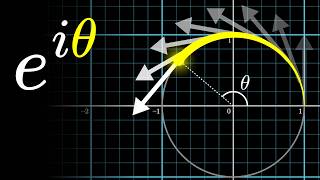

Why e^(iπ) = -1, Visualized
60sThis segment offers a stunning visual derivation of Euler's identity, a famous and often misunderstood equation, making it highly shareable.
▶ Play Clip"The title promises a physics-based explanation of Euler's formula, and the video delivers exactly that, with a clear and engaging visual approach."
This video is the first in a trilogy aimed at demystifying the Laplace transform, a powerful tool for solving differential equations. It focuses on building the foundational intuition for complex exponentials, e^(st), by exploring their geometric meaning and their role in solving physical problems like the damped harmonic oscillator. The video motivates why giving the exponent 's' complex values is natural and useful, setting the stage for the Laplace transform as a generalization of Fourier series.
This is the first video in a trilogy about the Laplace transform. It sets up the mental frameworks and prerequisite knowledge needed to understand the transform, which will be covered in the next two chapters.
The main characters are exponential functions, written as e^(st), where t is time and s is a number. The video aims to motivate why s should be allowed to take on complex values.
The derivative of e^t is itself. Visualizing this as a position on a number line, the velocity vector is always identical to the position vector, leading to accelerating growth.
For e^(-0.5t), the velocity is a 180-degree rotation of the position, scaled down. This results in an approach to zero at an ever-slowing pace.
For e^(it), the derivative is i times the function. Geometrically, multiplying by i is a 90-degree rotation, so velocity is always perpendicular to position, resulting in circular motion.
The circular motion traces one unit of arc length per unit of time. Waiting for π units of time lands halfway around the circle, explaining why e^(πi) = -1.
For complex inputs, e^x is just a notational shorthand for the Taylor series. Plugging in πi into the infinite polynomial results in a spiraling sum that converges to -1.
The imaginary part of s (ω) determines the frequency of oscillation, while the real part determines whether the magnitude grows or decays. Negative real parts correspond to exponential decay.
A central physics example: a mass on a spring. The force is proportional to position (Hooke's law), and a damping term proportional to velocity is often included. The goal is to find the position over time.
A bizarre trick is to guess that the solution is e^(st). This feels like knowing the answer ahead of time, but it leads to the Laplace transform.
Substituting e^(st) into the undamped oscillator equation gives s = ±i√(k/m). This introduces complex numbers, and the solution corresponds to oscillation in the complex plane.
To get a real-valued solution, add the two complex solutions. Due to linearity, the sum is also a solution, and it oscillates on the real number line like 2cos(ωt).
The equation is linear, so any linear combination of solutions is also a solution. The two complex solutions can be scaled and added to get the full family of solutions, including real-valued ones.
When damping is reintroduced, the solutions for s have both real and imaginary parts, leading to decay and oscillation. This is the damped harmonic oscillator.
For any linear differential equation with constant coefficients, substituting e^(st) leads to a polynomial in s. The fundamental theorem of algebra guarantees that this polynomial can be factored, giving a set of solutions.
Most real-world equations are not linear. For example, the driven oscillator in optics has a forcing term, and the solution is a combination of exponentials with specific coefficients, not freely tunable.
Exponentials e^(st) are like the atoms of calculus. Many functions can be broken up into these parts, making them simpler to study. This is especially true with infinite combinations over a continuum of s values.
The tool for finding these exponential parts is the Laplace transform. It extends the notion of Fourier series and transforms, applying to a much more general family of functions.
The Laplace transform translates functions into a new language where e^(st) are the fundamental units. Differentiation in time becomes multiplication by s, turning differential equations into algebra.
The video establishes the geometric and physical intuition for complex exponentials, showing how they naturally arise in solving differential equations. This sets the stage for the Laplace transform, which will be introduced in the next chapter as a tool to decompose functions into these exponential 'atoms'.
What is the derivative of e^(st) with respect to t?
s * e^(st)
13:28
Why does e^(πi) equal -1?
Because e^(it) traces a unit circle, and after π units of time, you are halfway around the circle, at -1.
05:29
What does the imaginary part of s represent in e^(st)?
It represents the frequency of oscillation.
07:46
What does the real part of s represent in e^(st)?
It represents whether the magnitude grows or decays (exponential growth or decay).
09:08
What is the general solution to the undamped harmonic oscillator equation?
A linear combination of e^(iωt) and e^(-iωt), where ω = √(k/m).
16:21
What is the key property of linear differential equations that allows adding solutions?
Linearity: any linear combination of solutions is also a solution.
16:48
What is the fundamental theorem of algebra?
Polynomials can always be factored as long as the roots are allowed to be complex numbers.
21:44
How does the Laplace transform simplify solving differential equations?
It turns differentiation into multiplication by s, transforming differential equations into algebraic equations.
26:41
Euler's Formula Explained
Provides a clear, geometric explanation of why e^(πi) = -1, a fundamental equation in mathematics.
05:29Complex Numbers Arise Naturally
Shows that solving a simple physics problem (mass on a spring) naturally introduces complex numbers, making them a necessary tool.
14:15Linearity and Real Solutions
Demonstrates how to combine complex solutions to get real-valued solutions, a key technique in solving differential equations.
16:21Exponentials as Atoms of Calculus
Introduces the powerful idea that many functions can be decomposed into exponential components, which is the foundation of the Laplace transform.
24:41Laplace Transform Preview
Highlights the core benefit of the Laplace transform: converting differential equations into algebraic ones, a huge simplification.
26:41[00:00] [Submit subtitle corrections at criblate.com] This is the first video in a trilogy aimed at demystifying the Laplace transform, a powerful tool for studying differential equations. Although we won't dig into the Laplace transform itself until the next two chapters,
[00:12] everything that we cover here sets up the mental frameworks and the prerequisite knowledge that make understanding that transform as easy as I know how. It's a very fun lesson in its own right about how one of the most
[00:27] famous equations in all of math is enables a bizarre trick for solving an equation that is used ubiquitously throughout physics. The main characters throughout this chapter and the next two are exponential functions,
[00:40] and I'm always going to be writing these as e^(st). Here we think of t as being time and then s as just some number determining which One of the big aims of this video is to motivate using physics why it's useful to
[00:57] give s the freedom to take on not only real number values, but complex ones as well. But wait a minute, what does it even mean to shove a complex number into an exponent? You see, there's some regular viewers of math videos online for whom the
[01:14] specific case of plugging in π times i is a little bit cliched by this point. It is amply covered by many videos on YouTube, but on the other hand, most students find this to be an understandably baffling notion.
[01:27] even if you fall into that first camp, I hope you'll agree that it's worth kicking things off here by reviewing a very beautiful and visual way to understand what this The nice part is that what follows doubles as a gentle warm
[01:43] up for visualizing and thinking about differential equations. You start with the fact that e to the t is its own derivative.
[01:55] Exponentials with other bases will have derivatives that are proportional to themselves, but e is the special number such that that proportionality constant is 1.
[02:07] Now, very often in a calculus class, you visualize derivatives as slopes of graphs. You should get in the habit of flexing your mind a bit more. position of some point on the number line as a function of time.
[02:22] Then what the derivative expression is telling you is that at every moment the velocity vector must look identical to the position vector. anything to the 0 is 1, you also have an initial condition.
[02:37] So at the very first moment, the velocity is also 1, meaning it's pointed to the right. But the farther to the right the position gets, the faster it must move. So even if you had never heard of the function e^t or exponential growth,
[02:52] this property alone is enough to give you a very visceral feeling for how it gives a value that grows and at an accelerating rate. But what if there was some constant in that exponent like e^(2t)?
[03:04] Well, by the chain rule, the derivative is then two times the function itself. velocity vector is always two times the position vector. But this time the feeling is that that growth gets out of hand all the more quickly.
[03:22] What if that constant was negative, say negative 0.5? Well, once again, by the chain rule, the derivative of So at every moment in time, that velocity vector looks like a 180 degree
[03:38] rotation of the position vector, but scaled down to be half its length. This means you start moving to the left, but as you approach zero with a smaller position vector, that velocity must get proportionally smaller.
[03:50] So it approaches zero, but at an ever slowing pace. But now for the fun part, why we're here in the first place. What if that constant was an imaginary number i, the square root of negative one?
[04:04] this function is going to be i times the function itself. Geometrically multiplying by i acts like a 90 degree rotation, so this is telling you velocity always has to be perpendicular to position.
[04:19] For anyone who's a little bit rusty or needs a quick review with complex numbers, which you typically draw in the 2D plane. by i is to go component-by-component.
[04:33] And then bi times i is b(i^2), which is -b. You'll notice each of those two individual components is rotated 90 degrees.
[04:48] So the sum as a whole also has to get rotated 90 degrees. evidently we must be thinking about position as being in the complex plane. Even if you had never heard of raising e to an imaginary number,
[05:02] and even if it's not clear at first what that would actually mean, the expression is telling you that this value has to move in such a way that the velocity vector is always locked to be a 90 degree rotated copy of the
[05:14] The only motion that satisfies this criterion is rotation around a circle, and you can be more specific because the initial position is 1, So this tells you how fast you have to move.
[05:29] it traces one unit of arc length for every unit of time. For example, to get one of the most famous equations in all of math, if you wait for π units of time, you end up precisely halfway around the circle.
[05:44] This is why e^(πi) is -1. confused by this expression is just how misleading the notation is. When you input a complex value, the expression really has very little
[05:58] not that much to do with the number e. The computation that it refers to is plugging in the input into this infinite polynomial, the Taylor series for e^x.
[06:10] It's actually very fun, I think, to take a moment to interpret the literal meaning of plugging in something like π times i for each one of these polynomial terms. As you take a higher power, each extra factor of i rotates you another 90 degrees,
[06:24] but then they shrink as that denominator takes over, and you end up with this spiraling sum that converges to minus one. Now, that said, it is not at all obvious, just looking at this infinite polynomial,
[06:39] you're going to end up walking around a unit circle. is a lot more helpful than focusing on the underlying computation.
[06:52] In practice, people get used to using the expression e^x as a notational shorthand here, Throughout this lesson, I'm going to be pulling up a complex plane representing possible values for this number s. And for each point on this plane,
[07:07] I want you to be able to think about the corresponding exponential function e^(st). We were just talking through what happens when s is equal to i. On the lower right I can show you how that output changes with time.
[07:19] And then on the top right, I might show a graph where, in order to fit it on the screen, I'll typically only graph the real part of that output with respect to time. If s is a different imaginary number, something like two i,
[07:33] And on the one hand, this is obvious. Throwing in a 2 in front of the time obviously moves you twice as fast. derivative expression is telling you dynamically.
[07:46] In this case, you can read it as saying the velocity is always a copy of the position vector rotated 90 degrees, but stretched to have a length of 2. More generally, it's common to label this imaginary part with the Greek letter omega,
[07:59] In other words, how many radians of arc length This is just the imaginary axis. But what about when s has both a real and an imaginary part?
[08:14] On the one hand, you can split up the exponential, And then this part is telling you that there's rotation.
[08:26] can think about it is to continue with the previous intuition. To understand what multiplication by any complex number looks like, you can ask what combination of rotation and stretching would place
[08:40] that would look like rotating a little over 90 degrees and stretching it out a bit. the relationship between the position and velocity vectors.
[08:54] way to see why the motion must be spiraling inwards. and which essentially means you should think of each point on that plane as encoding
[09:08] The imaginary part of s is always telling you how rapidly the function oscillates and in which direction. And then the real part of s is telling you whether the magnitude grows or shrinks.
[09:20] negative real parts corresponding to exponential decay. This key equation telling us that velocity is some modified version of position.
[09:32] And for you and me, having just seen how an intuition for reading off a differential equation like this can explain what complex exponents mean, at least if you want e^x to retain its core property.
[09:47] how a different set of differential equations can motivate why you would ever care about complex exponents in the first place. The easiest case to show you what I mean by this is a very central example
[10:01] used all throughout physics, where you imagine having a mass on a spring. We're going to describe the position of this mass as x, which will change over time. The derivative of this position versus time function,
[10:16] And then the second derivative, the rate of change of the velocity, The key feature of this spring setup is that the more you pull that spring to one side,
[10:28] the more strongly it accelerates the mass towards that equilibrium position. More specifically, we say that the force which is equal to mass times acceleration, that's Newton's second law, is often well approximated as k times the position.
[10:42] K here is just some positive proportionality constant. And this whole equation is telling you force is proportional to position. is because there are lots of other situations where you
[10:57] Often it's not exactly that, but as a first order approximation, It's also common to include a term here proportional to the velocity.
[11:09] This Greek letter mu is representing another positive coefficient. And the negative sign is telling you the faster this mass is moving, Maybe you think of it as friction, maybe you think of it as air resistance.
[11:24] that neither friction nor air resistance actually behave like this. But the better way to view it is that, again, this is a first order approximation of whatever the slowing forces might be on this mass.
[11:38] The position over time is an unknown function, And your physical intuition probably tells you loosely There's going to be some oscillation back and forth,
[11:53] the amplitude of that oscillation is going to decay. one side of it so that we're setting a bunch of stuff equal to zero.
[12:05] there's not one specific function that solves it, per se. you're going to get distinct functions that also solve the equation.
[12:18] because all of these are solutions where the initial velocity is zero. But you could also imagine that the mass starts out with some other non-zero velocity, and every one of these combinations of an initial position and initial velocity
[12:33] corresponds to a distinct function that also solves the equation. So to solve this, really you're looking for a family of functions that solve it. And preferably, you'd like some way to be able to narrow down which
[12:45] member of that family solves it for your specific initial conditions. Well, there's this one very bizarre trick which I remember really bothered me when I was a calculus student who first saw it, which is where you simply guess that the answer
[12:59] something that you're going to solve for. sort of just feels like asking the student to know the answer ahead of time.
[13:11] is probably not really how this mass on a spring behaves. But the point I want to make is that a desire to make this one of the things that leads you and me to the Laplace transform.
[13:28] Right here, let's just run forward and see what it gives us. then when you take its derivative, you. and then the second derivative again looks like the same function,
[13:45] but it's picked up another factor of s. And then all of the other constants just kind What's very nice here is that you can factor out that e^(st), and now everything that depends on time is tied up in this term right here.
[14:00] And moreover, exponentials will never equal zero. that this part right here has to equal zero. Solve this quadratic equation, one that looks kind of like a
[14:15] The easiest case here is if we ignore that damping coefficient. Basically setting mu equal to zero with a little bit of rearrangement and taking a square
[14:27] root, what you find is that s is going to be plus or minus the square root of -k/m. Now, k and m are both positive numbers, so that means, whether you wanted it or not, i, the square root of negative one, has now entered the game.
[14:42] This square root of k/m term is something that I'm going to give the suggestive shorthand name omega. And rolling back, remember what it is that s represents. We were exploring the possibility that a solution to this equation looks like e^(st).
[14:56] If we plug in these values for s, you now know what that means. corresponds to oscillation in the complex plane. Now, on the one hand, that is very weird because obviously our mass on
[15:10] But on the other hand, the idea of oscillating kind of matches what you want to find. Imagine that you increase that value k, meaning you have a stronger spring.
[15:24] And your physical intuition backs that up. A stronger spring probably would give you faster oscillation. Even still, the result, frankly, feels bizarre, if not obviously nonsense.
[15:38] I mean, the position of the mass on a spring is clearly a real number. And if you zoom out, really what's going on here is that we found for the pure there exists a complex valued function that solves it, namely e^(i * omega * t).
[15:55] To connect this pure mathland answer to something that's actually physical, you need to squeeze out a real valued solution from this. And the animation on screen kind of gives you one indication of how you could do this.
[16:07] real component of this solution that does actually work. But a better way to think about it, which will line up with the overall story I want to tell here that navigates towards Laplace transforms
[16:21] is to add up the two distinct complex solutions that we just found. the result stays constrained to the real number line. And in fact, the way that it oscillates on that number line over time looks
[16:35] like the function two times the cosine of that same frequency term times T. Now, the reason that you're allowed to just add two different solutions like this to get another solution is based on a critical property of our equation.
[16:48] distinct functions that solve it, then when you add up those functions, that sum of the two functions also solves the differential equation.
[17:00] If you scale each one of those functions by some constant and you add them up, that scaled sum is also a solution of the equation. just looking for one function or even two functions.
[17:15] solutions that will depend on the initial conditions. and the math came back to us with two distinct functions because it's linear,
[17:28] you can scale each one of those functions by some constant, add them together, And those scaling coefficients don't have to be real numbers. affects the initial angle of each of those rotating vectors.
[17:44] The family of all possible functions you can get by tuning these two coefficients is the family of all possible solutions to the original equation. But the real valued solutions are a special case of those.
[17:58] For example, if the initial position is supposed to be 2 and the initial velocity is supposed to be 0, then you get a valid answer by setting both of these coefficients
[18:10] to be 1, basically meaning you're just adding the two solutions we found earlier. then you simply scale both those constants by the same amount. Now, as presented so far, if this is supposed to be an example of why complex
[18:25] exponents are a natural and desirable thing, one of you could rightfully complain. If the so-called strategy is to just guess some function with a free parameter, it's not like it's hard to guess for this situation that a cosine or a sine would solve
[18:40] the equation, and you could have that frequency term be the free parameter that you're What you would find if you knew to make this guess, as long as you set that frequency to be the square root of k over m. And then,
[18:56] you can get the full family of solutions by scaling both of these and adding them And this is another valid way to describe the family of solutions. And you could argue this is a way more sensible coordinate
[19:13] Because in this case, all the real solutions are what you get simply by setting those scaling coefficients to be real numbers. Why complicate things with complex numbers?
[19:26] itself clear as soon as we try to generalize things. So far, when we solved for s, we got these two different values in the complex plane that are constrained to the imaginary line.
[19:40] you end up with different imaginary values that for your solution, correspond to distinct frequencies in the oscillation that you get. But think about what it means if we reintroduce that damping coefficient mu,
[19:54] Well, in this case, solving the equation looks like applying the quadratic formula. I'm just going to go ahead and show you what it looks like if
[20:08] I increase the value of that coefficient mu, and we see where the two corresponding solutions for S land in the complex plane. an imaginary but also a negative real component.
[20:21] And just a few minutes ago, we talked all about what it looks like if you want to exponentiate something with a negative real part and an imaginary part, it both does decays and oscillates, where the real part tells you how much it decays,
[20:34] In this case, what I'll do is graph for you the real component of that exponential, One thing that's actually pretty fun here is how if you increase that damping
[20:47] coefficient mu enough, eventually the solutions no longer have any imaginary part and they only have a real component, meaning the solution just looks like decay. This whole example is called the damped harmonic oscillator.
[21:02] so just understanding it in its own right is a worthy enough task. But how far does this dumb little trick actually take us? The straightforward way that you can generalize it is for any equation that looks
[21:16] you're scaling each one by some constant, you add them all up, In that case, everything we just did works essentially the same way.
[21:28] If you substitute e^(st) for x, then all of these derivative terms look just like that, This lets you factor out all of the exponential parts, leaving you with a certain polynomial in s that you want to equal zero.
[21:44] One of the most fundamental facts in algebra, literally called the fundamental theorem of algebra, is that polynomials can always be factored as long as you give those roots the freedom to maybe take on complex number values.
[22:02] your solutions might look something like this in the S-plane. Just like the oscillator example, this is basically the math telling you, hey, e^(st) can absolutely be a valid solution as long as you set s equal to one of these
[22:17] And just as before, this is a linear equation. each one of these exponentials and adding them together. All of these constants are like knobs and dials that you can tune to your heart's content.
[22:32] influence both the amplitude and the phase of each term. The specific values will depend on your initial conditions. but this is the general idea.
[22:46] Unfortunately, most real world equations are not simple linear ones like this. For example, the equation for a damped harmonic oscillator has actually come up on this channel before in a video about optics, but it came with a twist.
[22:59] We were studying why light appears to slow down in a medium like glass, And the key question was to understand why this depends on the color of that light, Now, I'm not going to recount all the details here,
[23:13] we were modeling charges inside the material, like glass, These little charges wiggling about some equilibrium position, an incoming light wave, which oscillated up and down as a sine wave.
[23:31] have nothing to do with the natural resonant frequency of the oscillator. but with this added term that looks like a certain cosine expression.
[23:44] Now, unlike the linear case, the family of solutions here does not can freely tune all of those constants to your heart's content. And this dumb trick of just guessing e^(st) certainly is not going to work.
[23:59] actually bring you a lot closer than you might expect. look like a combination of four specific exponentials.
[24:11] It's just that, unlike the linear case, you can't freely tune all of the coefficients. In fact, the whole substance of that prism example comes down to understanding exactly how big these coefficients are as a function of that incoming light frequency.
[24:26] differential equation that pops up in the real world looks like a certain combination of exponentials, but with particular coefficients. This ubiquity of exponentials is why engineers benefit from an intuitive understanding
[24:41] of points on the S-plane and how they can encode growth, decay, and oscillation. You can kind of think about these functions, e^(st) as being like the atoms of calculus.
[24:53] describe our world can often be broken up into these parts. And as long as you give s the freedom to take on complex values, and by breaking it up that way, they become simpler to understand and to study.
[25:06] This becomes especially true if you allow for infinite combinations, potentially over a continuum of values for s rather than some discrete set. We're going to go deep with that idea, and it is hard to overstate how powerful it is.
[25:19] The key question is, given some unknown function and a differential exponential parts like this, how do you actually find what those parts are?
[25:31] How would you know that the solution is built out of four specific exponentials? How would you solve for the appropriate values of s in the exponents? coefficients for a particular initial condition?
[25:46] There is a tool for this job, and as you may have guessed by this point, If you watched the earlier chapter about Fourier series, a lot of what I'm saying here is probably ringing all kinds of bells:
[25:59] Imaginary exponentials as describing a kind of rotation breaking up general functions And there is absolutely a connection here. A big part of the story I want to tell is how this Laplace transform
[26:12] we are building up to extends the notion of Fourier series and Fourier transforms, applying to a much more general family of functions. but here's a high level preview.
[26:24] When you use a Laplace transform to solve a differential equation, it actually ends up looking remarkably similar to that dumb trick of substituting e^(st). into algebra basically because the act of taking a derivative is
[26:41] the same as multiplication by s, at least for these specific functions. and it's for essentially the same reason too. What that operation does is translate functions into a new language where
[26:56] these terms e^(st), the atoms of calculus, are the fundamental units. Then again, the fact that differentiation in time looks like multiplication by derivatives start to look a lot like multiplication,
[27:12] and differential equations start to look like algebra. To see how exactly this transform is defined, how you can visualize what it's doing, come join me in the next chapter.
[27:27] chapter is available on Patreon, and my plan is to incorporate See you then.


⚡ Saved you 0h 27m reading this? Transcribe any YouTube video for free — no signup needed.